nextnano3 - Tutorial
next generation 3D nano device simulator
2D Tutorial
Efficient method for the calculation of ballistic quantum transport - The
CBR method (2D example)
Author:
Stefan Birner
If you want to obtain the input files that are used within this tutorial, please
check if you can find them in the installation directory.
If you cannot find them, please submit a
Support Ticket.
  -> 2D_CBR_MamaluySabathilJAP2003.in

 (-> 2D_CBR_MamaluySabathilJAP2003_holes.in -
same but for holes
instead of electrons)
==> Download nextnano³ CBR test executable:
2D_CBR_Mamaluy_SabathilJAP2003.zip
(If you don't have login and passwort yet, please
register here.)
Efficient method for the calculation of ballistic quantum transport - The
CBR method (2D example)
  -> 2D_CBR_MamaluySabathilJAP2003.in

 (-> 2D_CBR_MamaluySabathilJAP2003_holes.in -
same but for holes
instead of electrons)
In this tutorial we apply the Contact Block Reduction (CBR) method to a
Aharonov-Bohm-type structure where there is a large barrier in the middle of the
device.
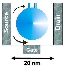
schematic sketch of the device showing two possible paths of the
electrons |
|
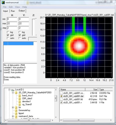
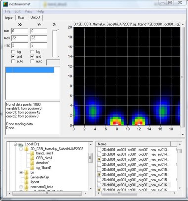
nextnanomat screenshot
(nextnanomat has been developed by Jörg
Ehehalt) |
This input file is based on the following paper:
[SabathilJAP]
Efficient method for the calculation of ballistic quantum transport
D. Mamaluy, M. Sabathil, P. Vogl
Journal of Applied Physics
93, 4628 (2003)
The device consists of three leads that are called 'source',
'gate' and 'drain'
in this example.
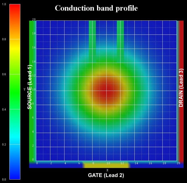
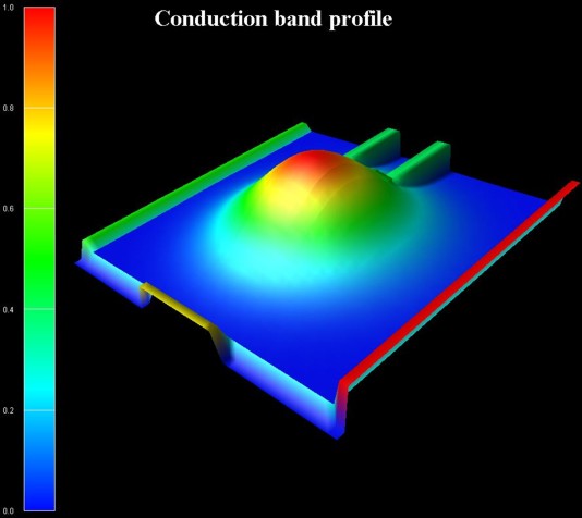
In the middle of the device a potential barrier of two-dimensional Gaussian
shape effectively expels the electrons from the center.
In the upper part of the device, a thin tunneling double barrier is present.
The device dimensions are 20 nm x 20 nm.
A detailed description of the device can be found in Section V. of
[SabathilJAP].
The effective electron mass is assumed to be constant throughout the device
and equal to 0.3 m0.
The device region consists of 41 x 41 = 1681 grid points, which is equivalent to
a grid spacing of 0.5 nm.
This means that the device Hamiltonian is a matrix of size 1681 x 1681.
The tunneling barriers have a width of 1 nm each and are separated by 3 nm.
The maximum height of the Gaussian barrier is Ec,0 = 1 eV, the height
of the double barriers is 0.4 eV.
The conduction band profile is given by Ec = Ec,0 exp[
- (x² + y²) / a² ] where x and y are with respect to the center of
the device,
and a = 5 nm.
The conduction band profile is achieved by using an appropriate ternary material
having a 2D Gaussian alloy profile.
The lower gate is 6 nm long, all other leads are 20 nm long.
The following figure shows the calculated transmission coefficients of the
various lead combinations T12, T23 and T13.
For the thick lines 18 % (303 of 1681) of all eigenvectors were used whereas for
the thin lines only 7 % (118 of 1681) had to be calculated, i.e. one does not
have to calculate all eigenvalues of the device Hamiltonian which grossly
reduces CPU time.
A small percentage of eigenvalues suffices for T(E) in relevant energy range of
interest.
The transmission coefficient can be found in this file:
CBR_data1/transmission2D_cb_sg001_ind000_CBR.dat
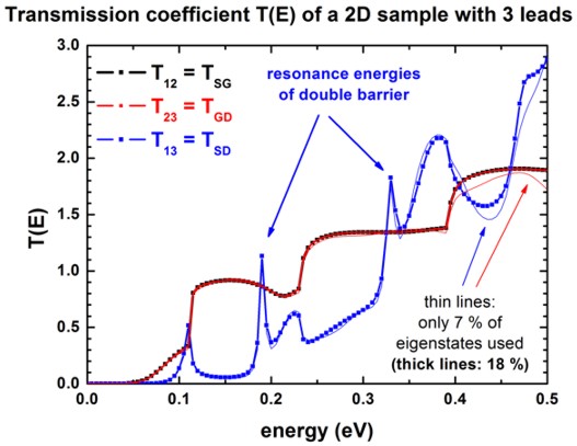
The nextnano³ results differ slightly from the [SabathilJAP]
paper.
Reason: The potential energy profile in the device and in the leads is not
exactly identical, as well as the dimensions of the barriers.
Therefore the eigenenergies and wave functions in the device, and in the leads
differ slightly which explains the small deviations.
==> The eigenstates # 16 is a resonance state of the
lower transmission path.
1st resonance: # 16: 0.123 eV
|
 |
|
nextnanomat screenshot
(nextnanomat has been developed by Jörg Ehehalt) |
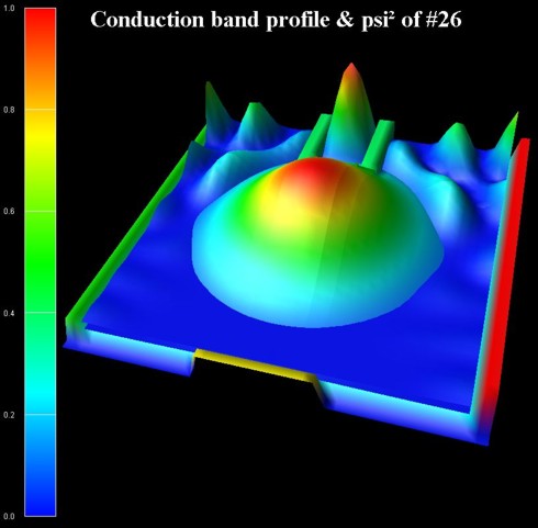
==> The eigenstates # 26 and # 29 are resonance states of
the double barrier.
1st resonance: # 26: 0.182 eV
(delocalized)
# 29: 0.196 eV (more localized)
2nd resonance: # 55: 0.322 eV (delocalized)
# 57: 0.333 eV (more localized)
# 60: 0.345 eV (delocalized)
# 63: 0.359 eV (more localized)
The following figure shows the conduction band profile together with the
square of the wave function of the 26th
eigenstate.
One can clearly see that it is a resonance state of the double barrier and
corresponds to the second peak in the blue transmission
curve T13 from source to drain around 180 meV.
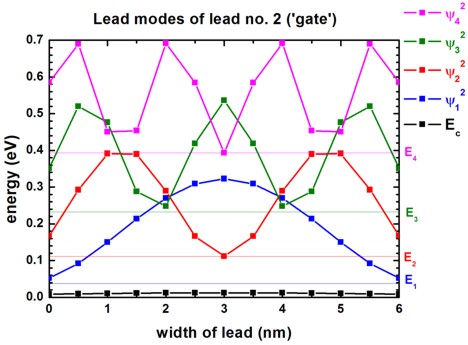
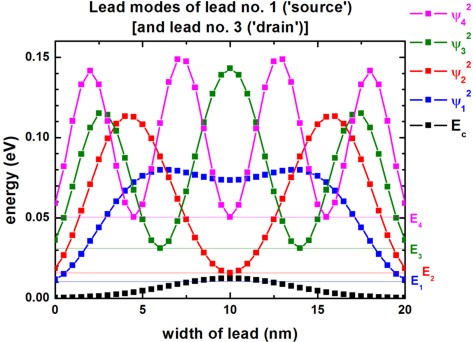
Lead modes
The following two figures show the lead modes of the gate, and the source
(which is identical to the drain).
In the transmission curve T12(E) = T23(E),
the transmission shows a step-like behavior which is related to the energies of
lead no. 2 ('gate').
The lead modes (eigenvalues, psi, psi², band edge profile, ...) can be found
in these files:
CBR_data1/modes_lead00*_sg001_*.dat
Technical details
Definition of contacts
For each contact (lead), a quantum cluster ("lead quantum cluster") has to be
defined because in each lead,
a one-dimensional Schrödinger equation has to be solved which gives us the lead
modes (i.e. energies and eigenvectors of the leads).
In addition, a quantum cluster is required for the device itself ("main quantum
cluster").
 !---------------------------------------------------!

 $quantum-regions
!


  region-number   = 1
! 'device'

  base-geometry   = rectangle
!

  region-priority = 2
!

  x-coordinates   = 0d0 20d0
! [nm]  width of 'device' = 20 nm

  y-coordinates   = 0d0 20d0
! [nm]  width of 'device' = 20 nm


  region-number   = 2
! 'source'

  base-geometry   = rectangle
!

  region-priority = 1
!

  x-coordinates   = -1d0 -0.5d0
! [nm]
(including 2 grid points along this direction)
  y-coordinates   =  0d0 20d0
! [nm]  length of 'lead 1' = 20 nm


  region-number   = 3
! 'gate'

  base-geometry   = rectangle                        !

  region-priority = 1
 !

  x-coordinates   =  7d0 13d0
! [nm]  length of 'lead 2' =  6 nm

  y-coordinates   = -1d0 -0.5d0
! [nm]
  region-number   = 4
! 'drain'

  base-geometry   = rectangle
!

  region-priority = 1
!

  x-coordinates   = 20.5d0 21d0
! [nm]
  y-coordinates   = 0d0
20d0
! [nm]  length of 'lead 3' = 20 nm


 $end_quantum-regions
!

 !---------------------------------------------------!
For each quantum cluster, the number of eigenstates to be calculated and its
boundary conditions have to be specified.
 !-------------------------------------------------!

 $quantum-model-electrons
!

  model-number
= 1
!

  model-name
= effective-mass  !
single band
effective-mass Schrödinger equation
  cluster-numbers
= 1

  conduction-band-numbers        =
1
!
 !number-of-eigenvalues-per-band = 118
!
  number-of-eigenvalues-per-band = 303
!
 !number-of-eigenvalues-per-band = 1681
!
  quantization-along-axes        =
1 1 0
!
  boundary-condition-100         =
Neumann
!
  boundary-condition-010         =
Neumann
!
For the main quantum cluster it holds:
If it is at the boundary, and if it is
in contact to a lead, a Neumann boundary condition is set.
If it is at the boundary, and if it is not in contact to a lead, a
Dirichlet boundary
condition is set.
 !-------------------------------------------------!

 ! lead 1 = source: number of modes per lead = 41
=
maximum number of relevant quantum grid points in lead 1
 !-------------------------------------------------!

  model-number
= 2
!

  ...

  cluster-numbers
= 2
!

  number-of-eigenvalues-per-band = 41
!
  boundary-condition-010         =
Dirichlet       !
 !-------------------------------------------------!

 ! lead 2 = gate:   number of modes per lead =
13 =
 !-------------------------------------------------!

  model-number
= 3
!

  ...

  cluster-numbers
= 2
!

  number-of-eigenvalues-per-band = 13
!
  boundary-condition-100         =
Dirichlet       !
 !-------------------------------------------------!

 ! lead 3 = drain:  number of modes per lead =
41 =
 !-------------------------------------------------!

  model-number
= 4
!

  ...

  cluster-numbers
= 2
!

  number-of-eigenvalues-per-band = 41
!
  boundary-condition-010         =
Dirichlet       !
 $end_quantum-model-electrons
!

 !-------------------------------------------------!
 !-------------------------------------------------!

 $CBR-current
!


!

  destination-directory = CBR_data1/
!
directory for output and data files
  calculate-CBR         =
yes
! "yes"/"no"
!
main-qr-num =
1
! number of main quantum cluster for which transport is calculated:
'device'

  num-leads
= 3
!
total number of leads attached to main region
  lead-qr-numbers       =
2  3  4
!
  propagation-direction = 1  2  1 !
'1'=x, '2'=y
! 1,2,3)
for each lead
  num-modes-per-lead    = 41 13 41
 !
! must be <= number of eigenvalues specified in
corresponding quantum model
 !num-eigenvectors-used = 118
!
  num-eigenvectors-used = 303
!
 !num-eigenvectors-used = 1681 !
1681=41*41=N_x*N_y!
  E-min
= 0.0d0
! [eV]
  E-max
= 0.5d0
! [eV]
  num-energy-steps      =
100
!
!

 $end_CBR-current
!

 !-------------------------------------------------!
For each energy E (num-energy-steps = 100)
where the transmission coefficient T(E) has to be calculated,
a matrix of size 95 x 95 has to be inverted.
The size of 95 is determined by the sum of the number of grid points in each
lead that are in contact to the device.
==> The total CPU time for calculation of the transmission
T(E) in this example was about 30 seconds for 303 eigenstates.
For further information, please study this section:
$CBR-current
|