CBR-current
This keyword is necessary for ballistic current calculations and for
calculations of the transmission coefficient T(E).
CBR = Contact Block Reduction method
Efficient method for the calculation of ballistic quantum transport
D. Mamaluy, M. Sabathil, and P. Vogl
J. Appl. Phys. 93, 4628 (2003)
Ballistic Quantum Transport using the Contact Block Reduction (CBR) Method -
An introduction
S. Birner, C. Schindler, P. Greck, M. Sabathil, P. Vogl
Journal of Computational Electronics 8, 267-286 (2009)
DOI 10.1007/s10825-009-0293-z
At a glance: CBR current calculation
- Full 1D, 2D and 3D calculation of quantum mechanical ballistic
transmission probabilities for open systems with scattering boundary
conditions.
- Contact Block Reduction method:
- Only incomplete set of quantum states needed (~ 10-20 %)
- Reduction of matrix sizes from O(N³) to O(N²)
- Ballistic current according to Landauer-Büttiker formalism
The CBR method is an efficient method that uses a
limited set of eigenstates of the decoupled device and a few propagating lead
modes to calculate the retarded Green's function of the device coupled to
external contacts. From this Green's function, the density and the current is
obtained in the ballistic limit using Landauer's formula with fixed Fermi levels
for the leads.
It is important to note that the efficiency of
the calculation and also the convergence of the results
are strongly dependent
on the cutoff energies for the eigenstates and lead modes. Thus it is important to
check during the calculation if the specified number of states and modes is
sufficient for the applied voltages. To summarize, the code may do its job very
efficiently but is far away from being a black box tool.
Limitation: A constant grid spacing in
real space is necessary. (It is possible to extend this algorithm to nonuniform
grids. Will be done in the future...)
!----------------------------------------------------!

$CBR-current
optional  !

 destination-directory      character
required  !
directory for output and
data files
 calculate-CBR
  character
optional ! yes"/"no"
 calculate-CBR-DOS
  character
optional ! yes"/"no"
 self-consistent-CBR        character
optional ! yes"/"no"
 read-in-CBR-states
  character
optional ! yes"/"no"
!

 main-qr-num
  integer
optional  !
 num-leads
  integer
optional  !
 lead-qr-numbers
  integer_array  optional
!
 propagation-direction      integer_array
optional  !
(1,2,3) for each lead
 num-modes-per-lead         integer_array
optional  !
!
num-eigenvectors-used integer_array optional !
 lead-modes-calculation     character
optional  !


!

 E-min
  double
optional  !
 E-max
  double
optional  !
 num-energy-steps
  integer
optional  !
 adaptive-energy-grid
  character
optional ! yes"/"no"
!

 extract-quasi-Fermi-level  character
optional ! yes"/"no"
!

$end_CBR-current
optional  !

!--------------------------------------------------!
Syntax
destination-directory = my-directory/


e.g. = CBR_data1/
Name of directory to which the files should be written. Must exist
and directory name has to include the slash (\
for DOS and / for UNIX)
calculate-CBR      = yes

                   =
no
Flag whether to calculate ballistic CBR current or not.
calculate-CBR-DOS  = yes

                   =
no
Flag whether to calculate and output the local density of states (which are
the diagonal elements (divided by 2 pi) of the spectral function), and the
density of states with the CBR method.
Note: The calculation of the transmission coefficient T(E) is much faster
than the calculation of the local DOS.
If one is only interested in the transmission coefficient, the calculation
of the local DOS can be omitted using this specifier.
self-consistent-CBR = yes

                    =
no   !
(default)
If yes, then the the quantum
density is calculated via the CBR method, and not by the usual quantum
mechanical approach (of occupying the square of the wave function with the
local quasi-Fermi level.)
This will influence self-consistent calculations.
See also adaptive-energy-grid.
read-in-CBR-states = yes

                   =
no    !
(default)
Flag whether to read in CBR states or not.
main-qr-num = 1
Number of main quantum cluster for which ballistic transport is calculated.
This cluster is usually labeled with 1
and corresponds to the device itself.
num-leads = 3  ! 2D/3D (>=
2)

num-leads = 2  ! 1D    (
must
be equal to 2 in 1D simulation)
Total number of leads (= contacts) attached to main quantum cluster (main-qr-num = 1).
In 1D, only 2 leads are possible.
For higher dimensions, more than 2
leads (= contacts) are possible.
2 leads is the lower boundary.
lead-qr-numbers = 2 3
Quantum cluster numbers corresponding to each lead.
Must be equal to "2 3"
for a 1D simulation.
propagation-direction = 1 1
Direction of propagation (1,2,3) for each lead.
1: along x direction
2: along y direction
3: along z direction
num-modes-per-lead = 41 13 41  !
2D/3D (
a value >= 1 is required
for each lead)
num-modes-per-lead = 1 1 !
1D (must be equal to "1 1"
for a 1D simulation)
Number of modes per lead used for CBR calculation.
Must be <= number of eigenvalues specified in corresponding quantum model.
Note: For k.p CBR calculation, one must take into account all
modes. For k.p, the number of modes per lead cannot be reduced.
For details about "Mode space reduction in single-band case", see section V.
in
Mamaluy et al., Physical Review B 71, 245321 (2005)
num-eigenvectors-used = 30 !
(This could be an integer array for each Schrödinger equation.)
Number of eigenvectors in main quantum cluster used for CBR calculation.
Must be <= number of eigenvalues specified in corresponding quantum model.
If number is larger than the number of eigenvalues specified in
corresponding quantum model, all eigenstates are used (default).
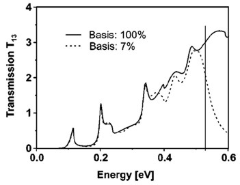
Example: The following figure shows the calculated transmission from
lead 1 to lead 3 as a function of energy T13(E).
Full line: All eigenfunctions (num-eigenvectors-used =
[maximum no. of eigenfunctions]) of the decoupled
device are taken into account.
Dashed line: Only the lowest 7% of the eigenfunctions are included (num-eigenvectors-used
= [0.07 * maximum no. of eigenfunctions]).
Here, Neumann boundary conditions are used for the propagation direction
at the contact grid points.
The vertical line indicates the cutoff energy, i.e. the highest eigenvalue
that is taken into account.
lead-modes-calculation = CBR-lead-Hamiltonian
!
(default)
= CBR-quantum-cluster !
= nextnano3-quantum-cluster ! (not
recommended so far)
This keywords specifies how
- for a 3D CBR (dim=3) calculation the 2D Schrödinger equation for
the leads is discretized to obtain the lead modes.
- for a 2D CBR (dim=2) calculation the 1D Schrödinger equation for
the leads is discretized to obtain the lead modes.
This keyword is only relevant for a 2D or 3D CBR calculation. It is irrelevant
for 1D CBR.
= CBR-lead-Hamiltonian
! Calculate eigenvalues and wave functions within CBR routine using a
separate Hamiltonian.
!
!
!
= CBR-quantum-cluster
! Calculate eigenvalues and wave functions within CBR routine
! using the nextnano³ implementation of the (dim-1) Schroedinger
equation.
! (only implemented for 2D CBR so far)
= nextnano3-quantum-cluster
! Take eigenvalues and wave functions from nextnano³ calculation.
! So far: (dim) Schrödinger equation is used, but: (to do) (dim-1)
Schrödinger equation should be used instead
In the long term, nextnano3-quantum-cluster
should be the default, or at least
CBR-quantum-cluster.
E-min = 0.0d0 ! 0.0 [eV]
Lower boundary for the energy interval of the transmission coefficient T(E) in units of [eV].
Should be smaller than the lowest eigenvalue E1.
E-max = 0.6d0 ! 0.6 [eV]
Upper boundary for the energy interval of the transmission coefficient T(E) in units of [eV].
If one wants to calculate the current for low temperatures, then it is
sufficient to set E-max to the energy of the Fermi level.
num-energy-steps = 100
Number of energy steps between E-min and E-max.
This number determines the resolution of the transmission curve T(E) where E
is the energy in units of [eV].
==> The number of energy grid points = num-energy-steps +
1
because the first grid point (E-min) is also included.
adaptive-energy-grid = adaptive-exponential
 !
(recommended for self-consistent CBR calculations)
= adaptive-linear       !


= adaptive-NEGF
 !
= no
 !
For self-consistent CBR (self-consistent-CBR = yes)
a self-adapting energy grid leads to faster convergence.
Information on the grid can be found in this file: EnergyGrid.dat
number of energy grid point energy [eV]
Note: The boundaries of the energy grid are automatically adjusted to
Emin = energy of lowest mode
Emax = + 0.2 eV
(Comment S. Birner: It might be necessary to adjust this value, or to use
as E-max the value specified in the input file.)
The remaining energy grid points are distributed over the grid to minimize
the maximum grid spacing.
 adaptive-exponential
/ adaptive-linear
:
This algorithm sets up the energy grid, trying to resolve the anticipated peaks in the density of states due to the onset of the lead modes (2D/3D).
In 1D, these are the band edge energies at the left and right device boundary.
This works particularly well in rather open devices,
where the density of (DOS) states is dominated by the leads.
The algorithm finds all propagating modes of a lead within an energy range
up to the lead cutoff and
resolves each mode by "points_per_mode" with a local grid spacing of delta_E
in an exponential or linear
grid
extract-quasi-Fermi-level = yes ! (default)
= no !
In a self-consistent CBR calculation, for the calculation of the density of
the bands that are not treated within the CBR method,
a quasi-Fermi level is required.
With this flag, an estimate is calculated.
For details, see the CBR paper of S. Birner et al.
Additional notes on the meaning of the quantum clusters
We need (at least) three quantum clusters, one for the device,
and the remaining for the leads.
Reason: We have to tell the nextnano³ code where the device Hamiltonian
and where the lead Hamiltonians have to be set up.
- quantum-cluster = 1: Device: This is the interesting region where we are solving
the Schrödinger equation of the device (decoupled device, i.e. closed
system).
Special boundary conditions for CBR method:
For the main quantum cluster (main-qr-num = 1)
for which ballistic transport is calculated, the nextnano³ code overwrites
internally the entries made in
the input file.
Generally speaking:
==>
==> Perpendicular to the propagation direction nextnano³ chooses Dirichlet.
(i.e. boundary condition for propagation direction: Neumann, for remaining
directions: Dirichlet)
Actually, to be more precise:
For each grid point in the main quantum cluster it is checked if
it is at the boundary and if it is in contact to a lead.
If it is at the boundary, and if it is
in contact to a lead, a Neumann boundary condition is set.
If it is at the boundary, and if it is not in contact to a lead, a
Dirichlet boundary
condition is set.
- quantum-cluster = 2: Lead no. 1: Dirichlet boundary conditions
perpendicular to propagation direction
- quantum-cluster = 3: Lead no. 2: Dirichlet boundary conditions
perpendicular to propagation direction
Note: Physically speaking, the lead quantum cluster must be a two-dimensional
surface in a 3D simulation, a one-dimensional line in a 2D simulation and a
zero-dimensional point in a 1D simulation.
So far the leads must contain 2 grid points along the propagation
direction. This is because it is currently not allowed to have a
two-dimensional (i.e. a width of 1 grid point only) quantum cluster in a 3D
simulation. Internally, the eigenvalues and modes are treated as to be
two-dimensional. In a 2D CBR simulation, similar restrictions apply, i.e. the
lead quantum regions must be rectangles of width 2 grid points, although
internally a one-dimensional line is used.
Note: The lead quantum cluster must not be overlapping with the device
quantum region. The lead quantum grid points must be neighbors to the device
quantum grid points.
Note: In the future, we will allow the user to specify 2D leads (rectangles)
in a 3D simulation, and 1D leads (lines) in a 2D simulation.
This is currently not possible.
Note: In 1D it is not necessary to specify more than one quantum cluster,
i.e. the quantum clusters for the leads must be omitted.
(For code developers: Check the specifier: lead-modes-calculation =
...)
Example
 $quantum-model-electrons

  model-number
= 1

  ...

  cluster-numbers        =
1         !
Main quantum cluster (main-qr-num = 1)
for which ballistic transport is calculated.
boundary-condition-100 = Dirichlet !
This boundary conditions is overwritten internally in any case.
boundary-condition-010 = Dirichlet !
boundary-condition-001 = Neumann !
(propagation direction is along z direction)
  model-number
= 2

  ...

  cluster-numbers        =
2         !
  boundary-condition-100 = Dirichlet !

  boundary-condition-010 = Dirichlet !

  boundary-condition-001 = Neumann   !
  model-number
= 3

  ...

  cluster-numbers        =
3         !
  boundary-condition-100 = Dirichlet !

  boundary-condition-010 = Dirichlet !

  boundary-condition-001 = Neumann   !
Note: The boundary conditions are irrelevant. They are overwritten
internally.
The CBR method only works if you have chosen the correct flow-scheme ($simulation-flow-control).
The current cluster must be deactivated.
 $current-cluster

  cluster-number     = 1

  region-numbers     = 1

  deactivate-cluster = yes
In order to print out current-voltage characteristics (I-V characteristics), the
corresponding specifier must be activated, see
$output-current-data
for details.
Output
- Transmission coefficient Tij(E) between Lead i and Lead j of
Schrödinger equation
sg001
- transmission2D_cb_sg001_CBR.dat

  Energy[eV]    T_01_02    T_01_03
	T_02_03
- Density of states DOS(E) for each lead, and the total DOS(E)
	- DOS1D_sg001.dat

  energy[eV]   Lead001   Lead002
	SumOfAllLeads
[eV^-1].
- (Total) local density of states LDOS(z,E), i.e. sum of LDOS(z,E) of each
lead
- LocalDOS1D_sg001.dat / *.coord / *.fld *_ij.dat
format ( x,y, f(x,y) )
position[nm] energy[eV] LDOS[eV^-1nm^-1]
The units of the LDOS are [eV^-1 nm^-1].
- In 1D, the LDOS(z,E) is a two-dimensional plot.
How the hell do I plot these strangely
".dat / *.coord / *.fld"-like formatted files?
-
-
- Local density of states LDOS(z,E) of each lead
- LocalDOS1D_sg001_Lead01.dat / *.coord / *.fld
*_ij.dat format ( x,y, f(x,y) )
position[nm] energy[eV] LDOS[eV^-1nm^-1]
The units of the LDOS are [eV^-1 nm^-1].
- In 1D, the LDOS(z,E) is a two-dimensional plot.
How the hell do I plot these strangely
".dat / *.coord / *.fld"-like formatted files?
-
-
- Additional 1D output:
Local density of states LDOS(z=zmin,E) and LDOS(z=zmax,E) at the boundaries
of the device (i.e. at contact grid points).
- LocalDOS_at_boundaries1D_sg001.dat
energy[eV] LDOS(zmin,E)[eV^-1nm^-1] LDOS(zmax,E)[eV^-1nm^-1]
- Energy grid that is used for the CBR calculation
- CBR_EnergyGridV.dat

  EnergyGridPoint    Energy[eV]
The energy grid could have a constant grid spacing, or be a
self-adapting grid with varying grid spacing.
- Electron or hole density as calculated from the CBR algorithm
1D:
- density1D_sg001.dat

  position[nm]   density[10^18cm^-3]
2D:
- density2D_sg001.dat / *.coord / *.fld or in the
*_ij.dat format ( x,y, f(x,y) )
position[nm] density[10^18cm^-3]
3D:
- density3D_sg001.dat / *.coord / *.fld or in the
*_ijk.dat format ( x,y,z, f(x,y,z) )
position[nm] density[10^18cm^-3]
- Fermi levels
	- _FermiLevel_el_CBR.dat

	- _FermiLevel_hl_CBR.dat

  position[nm]   FermiLevel[eV]
Parallelization of CBR algorithm
The CBR algorithm has been parallelized, i.e. the
loop over num-energy-steps.
This is relevant for 2D and 3D CBR calculations, in 1D the effect is very small
(negligible).
Three options for parallelization are available.
-
no parallelization
-
parallelization with
OpenMP (executables
compiled with Intel compiler, including parallel version of MKL)
Very easy to use, i.e. specify number of parallel threads via command line:
nextnano3.exe -threads 4
(uses four threads, e.g. on a quad-core CPU)
-
parallelization with
Coarray Fortran
(executable compiled with g95
compiler)
Not so easy to use, only available on Linux so far:
Start g95 Coarray console:
 cocon

 fork 4
run nextnano3_g95.exe
For further details, see also:
  $global-settings

   ...

   number-of-parallel-threads = 2
! 2 =
for dual-core CPU
|