|
| |
Output-file-format
There are several options for 1D, 2D and 3D. You can specify the desired
output file format to suit your favorite visualization software package.
We recommend to first try it with our in-house visualization software
nextnanomat.
All nextnano output is with respect to a rectilinear grid.
1D
2D
3D
!------------------------------------------------------!

$output-file-format
optional !

 simulation-dimension
integer
required ! CHOICE[1,2,3]

 gnuplot
character
optional ! CHOICE[no,yes]

 VTK-XML
character
optional ! CHOICE[yes,no]

 VTK-legacy
character
optional ! CHOICE[no,yes]

 AVS-Express
character
optional ! CHOICE[no,yes]

 number-of-AVS-files
integer
optional ! CHOICE[1,2,3]

 file-format
character
optional ! CHOICE[Origin,ASCII,AVS-ASCII,AVS-binary,AVS-binary-single,AVS-binary-double]

 resolution
character
optional ! CHOICE[default,average,all]
only 2D/3D
$end_output-file-format
optional !

!------------------------------------------------------!
Syntax
!------------------------------------------------------!

$output-file-format
!


!

 simulation-dimension = 1
!
1D
 file-format          =
Origin
! (ASCII format + *.plt Origin files)

!file-format          =
ASCII
! (ASCII format)


 simulation-dimension = 2
!
!

 VTK-XML
= yes

! .vtr, r = rectilinear
grid)
 VTK-legacy           =
no

! .vtk)
!

 AVS-Express
= yes

! .fld) (default)
!

 file-format          =
AVS-ASCII
!
!file-format          =
AVS-binary
!
AVS-binary-single

!file-format          =
AVS-binary-single
!
AVS/Express (Fortran's binary format, i.e. 'unformatted' in single
precision)
!file-format          =
AVS-binary-double
!
!

 resolution           =
default
! default / all / average


 simulation-dimension = 3
!
... simulation-dimension = 2
!
$end_output-file-format
!
!------------------------------------------------------!
The file size of
AVS-binary-single *.dat
files is only half the size of AVS-binary-double.
AVS-binary-single/AVS-binary-double
is much faster than AVS-ASCII,
especially for large arrays of data.
 gnuplot
= yes

! output *.gnu.plt and *.ij.ijk files to be plotted with gnuplot


= no

!
Gnuplot
$output-file-format


 simulation-dimension = 1

 gnuplot
= yes !
Output gnuplot files for 1D plots such as E_c(x).
!gnuplot
= no  !
 simulation-dimension = 2

 gnuplot
= yes !
!gnuplot
= no  !
$end_output-file-format
 VTK-XML
= yes

!
VTK XML ASCII format (.vtr, r = rectilinear
grid)
= no

!
 VTK-legacy           =
yes

! .vtk)
= no

!
==> VTK - The
Visualization Toolkit
The .vtr format can be read by the following software:
AVS/Express format for rectilinear grid
 AVS-Express
= yes

!
AVS/Express ASCII format (.fld) (default)
= no

!

==>
 number-of-AVS-files  = 1
! .fld
file
- Everything is written into the .fld file. (default)
= 2
! .fld,          .dat
- The .coord information is put into the .fld
file.
= 3
! .fld, .coord., .dat
= 4
! .fld, .coord., .dat .v file is
written out. It is related to the AVS/Express software.
Resolution
In
2D/3D you can
additionally specify, how many points you want to plot (resolution) in order to
make large amounts of visualization data to be handled more efficiently.
In 2D, for each point on material grid, 4 octants are created each containing one
point (only relevant for grid lines at interfaces).
In 3D, for each point on material grid, 8 octants are created each containing
one point (only relevant for grid lines at interfaces).
 resolution
= default
!
                      =
all
!
=
average
!
! ==>
default will plot
multiple points at material interfaces where useful, e.g. for conduction band
edges or valence band edges where there are abrupt steps at interfaces.
In cases where this is not necessary (e.g. for electrostatic potential,
wave functions, ...), no multiple points are written out unless
all is chosen..
1D
x, f(x)
That's plane ASCII, suitable for everything.
2D
x, y, f(x,y)
- Output files that will be produced are:
- The output files can be read in with the AVS/Express software that can be
obtained by Advanced Visual Systems.
AVS output files described in the next three paragraphs:
- material_grid.fld
- material_grid.coord
- material_grid.dat
- material_grid.fld
This is an AVS field file specifying the input files and data format
needed for processing the 2D/3D visualization.
# AVS field file        !

  #                       !

  ndim   =  2             !
dimension of data
dim1 = 46 !
dim2 = 112 !
nspace = 2 !
veclen = 1 !
data = float ! integer / float / double (integer
precision / single-precision real number / double-precision real number)
field = rectilinear !
label = material_grid !
  variable 1 file=material_grid.dat   filetype=ascii       skip = 0     offset = 0   stride=1
	!
 file-format =
AVS-ASCII

	variable 1 file=material_grid.dat   filetype=unformatted skip = 0     offset = 0   stride=1
	!
if file-format =
AVS-binary
coord 1 file=material_grid.coord filetype=ascii skip = 0 offset = 0 stride=1
coord 2 file=material_grid.coord filetype=ascii skip =
112 offset = 0 stride=1 !
As an empty line separates the coordinate axes, we have 112 + 1 =
113.
The x coordinates are located at position 0 to 112 in the file material_grid.coord, y coordinates are located in the same file at position
112 to 158.
The variable data is stored in the .dat file and is related to
the coordinates in a systematic order.
Note:
Fortran 'unformatted' data is binary data with additional words (of length 4
bytes) written at the
beginning and end of each data block stating the number of bytes or words in the
data block.
More information on the .fld type can be found
here.
- AVS input files:
material_grid.coord, material_grid.dat
- material_grid.coord
Coordinates of the grid, i.e. 112+46 real numbers that
specify the grid points on each axis. - material_grid.dat
Contains information about the regions.
Each grid point is specified by a region number as defined in the input
file (see table at top of this page). - All other folders contain the same structure for AVS field files:
- *.fld
- *.coord
- *.dat
3D
x, y, z, f(x,y,z)
- The output files can be read in with the AVS/Express software that can be
obtained by Advanced Visual Systems.
AVS output files described in the next three paragraphs:
- material_grid.fld
- material_grid.coord
- material_grid.dat
- material_grid.fld
This is an AVS field file specifying the input files and data format
needed for processing the 3D visualization.
# AVS field file        !

  #                       !

  ndim   =  3             !
dimension of data
dim1 = 53 !
dim2 = 53 !
dim3 = 70 !
nspace = 3 !
veclen = 1 !
data = float ! integer / float / double (integer
precision / single-precision real number / double-precision real number)
field = rectilinear !
label = material_grid !
  variable 1 file=material_grid.dat   filetype=ascii       skip = 0    offset = 0  stride=1
	!
 file-format =
AVS-ASCII

	variable 1 file=material_grid.dat   filetype=unformatted skip = 0    offset = 0  stride=1
	!
if file-format =
AVS-binary
coord 1 file=material_grid.coord filetype=ascii skip = 0 offset = 0 stride=1
coord 2 file=material_grid.coord filetype=ascii skip =
70 offset = 0 stride=1 !
As an empty line separates the coordinate axes, we have 70 + 1 =
71.
  coord 3    file=material_grid.coord filetype=ascii       skip =
	123  offset = 0  stride=1  !
125.
The x coordinates are located at position 0 to 70 in the file material_grid.coord, y coordinates are located in the same file at position 71
to 123, ...
The variable data is stored in the .dat file and is related to
the coordinates in a systematic order.
Note:
Fortran 'unformatted' data is binary data with additional words (of length 4
bytes) written at the
beginning and end of each data block stating the number of bytes or words in the
data block.
- AVS input files:
material_grid.coord, material_grid.dat
- material_grid.coord
Coordinates of the grid, i.e. 53+53+70 real numbers that
specify the grid points on each axis. - material_grid.dat
Contains information about the different materials used in the simulation.
Each grid point is associated with a certain material number as defined in
the input file.- All other folders contain the same structure for AVS field files:
- *.fld
- *.coord
- *.dat
The data values are written to the .dat file in the following
order:
   DO   k=1,dim3

    DO  j=1,dim2

     DO i=1,dim1

        WRITE(*,*)
matrixM(1:DimVector,i,j,k) ! DimVector = 1 for scalar quantity

     END DO

    END DO

   END DO
- You must have three files in your directory:
your_filename.fld
your_filename.coord, your_filename.dat
- Use this perl script:
avs2xyz.pl (avs2xyz_pl.zip)
Usage: avs2xyz.pl
your_filename
- Output that will be created (containing three columns:
x, y, f(x,y)):
your_filename.xyz
On the screen there will be some output about the number of x and y
coordinates (you will need it later!).
- Open Origin.
- Import
your_filename.xyz to an
Origin worksheet.
- Mark the third column as Z.
- Mark third column.
- Column -> Set as Z
Worksheet -> Convert to Matrix -> Random XYZ ->


  No. of columns  = no. of x grid coordinates


  No. of rows     = no. of y grid coordinates
  Gridding method = Weighted average or


  Correlation
Plot3D -> 3D Colormap Surface (for
instance)- If the Origin plot doesn't satisfy you, there are some ways around to
improve it. We are not experts in that but maybe you could contribute to
improve this documentation with your know-how. Many thanks!
Some hints:
- Right mouse button
   -> Layer Contents...

      -> Layer Properties

-> Size/Speed -> Skip Points" (to show all/more points)
-> Axis -> Length ->
type in x and y real scale values (to scale properly)
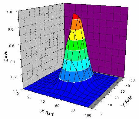
- Example (2D wave function):
AVS/Express Hints
=> Turn the (default) black background color into a white
background color:
-> Editors -> View -> General -> Background Color Editor -> Set
Value to 1.0.
=> Change line thickness (of e.g. orthoslice):
	-> Select: Editors -> Object -> Properties -> Type -> Point/Line -> Line
	Thickness -> ...
|