|
| |
nextnano3 - Tutorial
next generation 3D nano device simulator
1D Tutorial
Quantum-Cascade Laser
Author:
Stefan Birner
If you want to obtain the input files that are used within this tutorial, please
check if you can find them in the installation directory.
If you cannot find them, please submit a
Support Ticket.
-> 1DQuantumCascadeLaser.in

    -> 1DQCL_AlGaAs_Sirtori_APL73_1998.in

    -> 1DQCL_Andrea_Friedrich_NoInjector_InGaAs_APL86_2005_77K_kp.in

    -> 1DQCL_Andrea_Friedrich_NoInjector_InGaAs_APL86_2005_300K_kp.in

    -> 1DQCL_Rochat_APL81_2002.in

    -> 1DQCL_THz_MIT_Sandia_SemicScTech20_2005.in

    -> THzQCL_Andrews_Vienna_MatSciEng2008_nn3.in / *_nnp.in -
input file for nextnano³
and nextnano++ software
    -> 1DQuantumCascadeLaserSiGe_nn3.in
/ *_nnp.in - |
Quantum-Cascade Laser
This tutorial is based on the quantum-cascade structure that has been
presented in the following paper.
300 K operation of a GaAs-based quantum-cascade laser at lambda=9 µm
H. Page, C. Becker, A. Robertson, G. Glastre, V. Ortiz, C. Sirtori
Applied Physics Letters 78 (22), 3529 (2001)
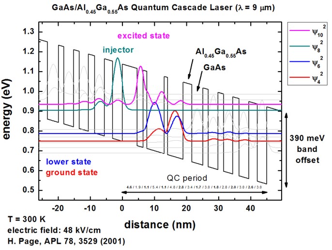
Here, we are trying to reproduce Fig. 1 of this paper.
The temperature has been set to 300 K.
The quantum-cascade structure consists of a sequence of GaAs wells and Al0.45Ga0.55As
barriers. The sequence is as follows (from 0 nm to 45 nm; it is repeated outside
this region):
4.6 / 1.9 / 1.1
/ 5.4 / 1.1 / 4.8 /
2.8 / 3.4 / 1.7 / 3.0 /
1.8 / 2.8 / 2.0
/ 3.0 / 2.6 / 3.0
The units are [nm]. Blue and bold
scripts indicate Al0.45Ga0.55As
barriers, normal scripts indicate GaAs wells.
In the APL paper, a conduction band offset of 390 meV was used.
Consequently, we modify our default band offset by shiftting the AlGaAs ternary
slightly to also get 390 meV.
 $ternary-zb-default

  ternary-type = Al(x)Ga(1-x)As-zb-default

  ...

  band-shift   = 0.022719d0
! [eV]
==> to get a band offset of 390 meV for T=300 K and x=0.45 (Al0.45Ga0.55As)
We apply an electric field of -48 kV/cm:
 $electric-field
!

  electric-field-on        =
yes    ! 'yes'
/ 'no'

  electric-field-strength  = -48d5
! [V/m] - Here: -48 kV/cm
electric-field-direction = 0 0 1 !
[001] direction, i.e. along z axis.
$end_electric-field
!
For simplicity, in contrast to the APL paper, we do not include doping here.
In the original APL paper, the following areas were n-type doped with silicon
with a sheet density of nSi = 3.8 * 1011 cm-2.
=> between 15.2 nm and -5.6 nm (9.8 nm): '1.8 nm' (barrier), '2.8
nm' (well), '2.0 nm' (barrier) and '3.0 nm' (well)
=> between 29.8 nm and 39.4 nm (9.8 nm): '1.8 nm' (barrier), '2.8
nm' (well), '2.0 nm' (barrier) and '3.0 nm' (well)
We use flow-scheme = 21.
$simulation-flow-control
 ! flow-scheme = 20   ! ==> apply
electric field and        solve Poisson
equation
   flow-scheme = 21   ! ==>
apply electric field and do not solve Poisson equation
...
These flow-schemes includes the following:
1. Calculate the strain (if any).
2. Calculate the piezo and pyroelectric charges (if any).
3. Calculate the conduction and valence band edge profiles by solving Poisson's
equation taking into acount doping (if any), piezo and pyroelectric charges (if
any) and deformation potentials (if strain unequal to zero).
4. Apply the electric field.
5. Calculate the eigenstates and wave functions by solving Schrödinger's equation
(either single-band or k.p).
Note that for flow-scheme = 21, this
is not a self-consistent calculation of the Poisson-Schrödinger equation.
flow-scheme = 20 is self-consistent
but a severe limitation is that population inversion is not taken into account.
In our example, we did not have to calculate the strain. Piezo any
pyroelectric fields do not exist. We do not include doping. We used single-band
(effective-mass) rather than 8-band k.p.
The following figure shows the conduction band energy of the Gamma conduction
band edge and the wave functions (psi² = psi squared) of the
ground state 1, the
lower state 2, the excited state 3
and the injector state i.
|
 |
|
The figure shows the conduction band edge (black
line) of the quantum-cascade structure that has a slope because of the
electric field of -48 kV/cm.
Also shown are four wave functions (psi² = psi squared) that are shifted by
their corresponding eigenenergies. |
The above shown structure of the conduction band edge and the wave functions
is in excellent agreement with Fig. 1 of the following paper:
300 K operation of a GaAs-based quantum-cascade laser at lambda=9 µm
H. Page, C. Becker, A. Robertson, G. Glastre, V. Ortiz, C. Sirtori
Applied Physics Letters 78 (22), 3529 (2001)
Note that periodic boundary conditions for the Schrödinger and Poisson
equation do not make sense because of the application of an electric field. Thus
we used Dirichlet boundary conditions. However, this will lead to some
artificial, wrong wave functions at the boundaries because the wave function is
forced to be zero at the boundaries. For the states in the middle of the device
where the wave function decays to zero in any case at the boundaries, the
boundary conditions do not have any influence at all and so these states are
fine.
So the suggestion is to calculate 3 or 5 periods, and then take the energy
levels and wave functions of the center period.
In this way, boundary effects should not be very severe.
 $quantum-model-electrons

   model-number
= 1

   model-name
= effective-mass  ! 'effective-mass'
or '8x8kp'
boundary-condition-001 = Dirichlet !
boundary condition for [001] direction, i.e. along the z
direction
...
Intraband matrix elements
The files
- Schroedinger_1band / intraband_pz1D_cb001_qc001_sg001_deg001_dir.txt and
- Schroedinger_1band / intraband_z1D_cb001_qc001_sg001_deg001_dir.txt
Our result for the excited state to
lower state 'z' matrix element is in
excellent agreement with the result of [Page]:
Intersubband dipole moment  | < psi_f* | z | psi_i > |  [nm]

------------------|----------------------------------------------------------------------


Oscillator strength []

------------------|--------------|-------------------------------------------------------


Energy of transition [eV]

------------------|--------------|-------------|-----------------------------------------


m* [m_0]      lifetime [ps]

------------------|--------------|-------------|-------------|-------------|-------------

...

<psi010*|z|psi006>
1.6655138016  0.747520328
0.147729769   0.069499455


==> z10,6
= 1.6655138016 [nm]
([Page] : z32
= 1.7 nm)
The transition energy of these two states has been calculated to be
147.7 meV. ([Page, Fig. 3, experiment] : E32
= 160 meV)
For more details, check the tutorial on intraband transitions:
Optical intersubband transitions
in a quantum well - Intraband matrix elements and selection rules
QCL examples
Note: We have nextnano³ input files available for
quantum-cascade lasers that are based on the following structures.
Please submit a support ticket
if you want to obtain these input files.
- 9 µm, i.e. 33 THz or 138 meV
300 K operation of a GaAs-based quantum-cascade laser at lambda=9 µm
H. Page, C. Becker, A. Robertson, G. Glastre, V. Ortiz, C. Sirtori
Applied Physics Letters
78 (22), 3529 (2001)
-> 1DQuantumCascadeLaser.in
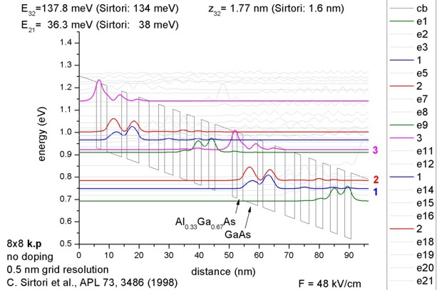
- 9.4 µm or 132 meV
GaAs/AlxGa1-xAs quantum cascade lasers
C. Sirtori, P. Kruck, S. Barbieri, P. Collot, J. Nagle, M. Beck, J. Faist, U.
Oesterle
Applied Physics Letters 73 (24), 3486 (1998)
-> 1DQCL_AlGaAs_Sirtori_APL73_1998.in
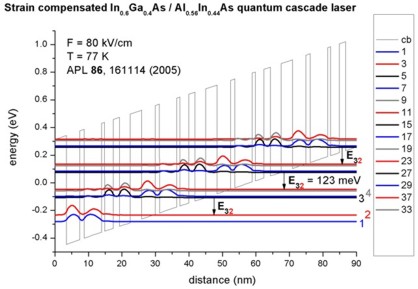
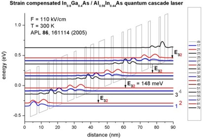
- 10 µm, i.e. 124 meV (77 K)
8.4 µm, i.e. 148 meV (300 K)
Quantum-cascade lasers without injector regions operating above room
temperature
A. Friedrich, G. Böhm, M.C. Amann, G. Scarpa
Applied Physics Letters
86, 161114 (2005)
-> 1DQCL_Andrea_Friedrich_NoInjector_InGaAs_APL86_2005_77K_kp.in

  -> 1DQCL_Andrea_Friedrich_NoInjector_InGaAs_APL86_2005_300K_kp.in
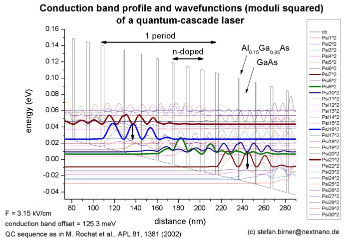
- 66 µm, i.e. 4.54 THz or 18.8 meV (nextnano³ calculation:
18.5 meV, i.e. 4.47 THz or 67 µm)
Low-threshold terahertz quantum-cascade lasers
M. Rochat, L. Ajili, H. Willenberg, J. Faist, H. Beere, G. Davies, E.
Linfield, D. Ritchie
Applied Physics Letters 81 (8), 1381 (2002)
-> 1DQCL_Rochat_APL81_2002.in
Note: The caption in FIG. 1 in this paper must read "from right to left",
rather than "from left to right".
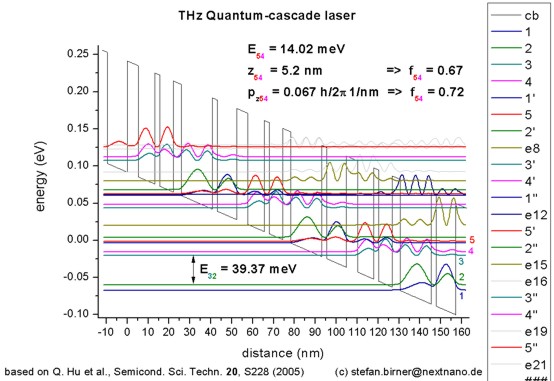
- 89.2 µm, i.e. 3.4 THz or 13.9 meV (exp. 14.2 meV) (nextnano³ calculation:
14.02 meV)
Resonant-phonon-assisted THz quantum-cascade lasers with metal-metal
waveguides
Q. Hu, B.S. Williams, S. Kumar, H. Callebaut, S. Kohen, J.L. Reno
Semiconductor Science and Technology
20, S228 (2005)
-> 1DQCL_THz_MIT_Sandia_SemicScTech20_2005.in
- 107 µm, i.e. 2.8 THz or 11 meV
Doping dependence of LO-phonon depletion scheme THz quantum-cascade
lasers
A. M. Andrews, A. Benz, C. Deutsch, G. Fasching, K. Unterrainer, P.
Klang, W. Schrenk, G. Strasser
Materials Science and Engineering B 147, 152 (2008)
-> THzQCL_Andrews_Vienna_MatSciEng2008_nn3.in - input file for
nextnano³ software
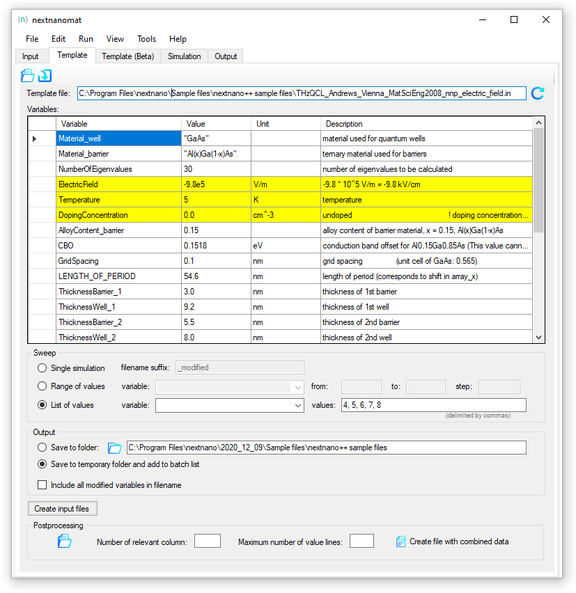
-> THzQCL_Andrews_Vienna_MatSciEng2008_nnp.in -
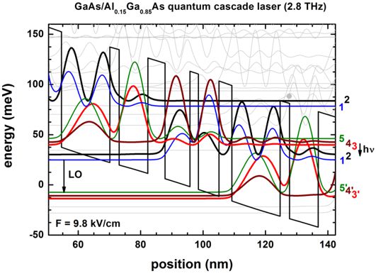
This input file is parameterized. One can thus use nextnanomat's
Template feature to vary e.g. alloy content or barrier widths.
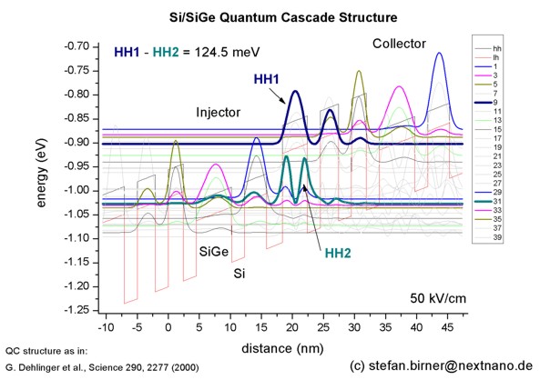
- 9.9 µm, i.e. 30.2 THz or 125 meV (nextnano³ calculation:
124.5 meV)
Intersubband Electroluminescence from Silicon-Based Quantum Cascade
Structures
G. Dehlinger, L. Diehl, U. Gennser, H. Sigg, J. Faist, K. Ensslin, D.
Grützmacher, E. Müller
Science 290, 2277 (2000)
-> 1DQuantumCascadeLaserSiGe?nn3.in
Note: The Science article reports a calculated transition energy of 130 meV.
The experimentally measured value, however, was reported to be 125 meV which
is in excellent agreement with the nextnano³ calculations based on the
default parameters in the nextnano³ database.
The eigenstates relevant for the optical transitions are the numbers 9 & 10,
and 31 & 32.
|