|
| |
Import data on material-grid
Imports data from arbitrary rectilinear grid onto simulation grid:
- 1D: linear interpolation
- 2D: bilinear interpolation
- 3D: trilinear interpolation
Here, the term "material-grid" does not necessarily mean "material grid". E.g. the
electrostatic potential and the Fermi levels are mapped onto the physical grid,
and not onto the material grid. The strain is mapped onto the material grid.
This feature works for 1D, 2D and 3D simulations.
The subroutines read in ASCII data of format coordinates,
data[1,...,n] with a blank as a separator, i.e.
1D:
    x1
f(x1)

    x2
f(x2)

    ...
    x1  y1
f(x1,y1)

    ...
    x1  y1  z1
f(x1,y1,z1)

    ...
f can also be a vector (which is
necessary for the strain tensor which has n=6 independent
components).
  x1
f_1(x1)       ...  f_n(x1)
2D: x1 y1
f_1(x1,y1) ... f_n(x1,y1)
3D: x1 y1 z1 f_1(x1,y1,z1) ...
f_n(x1,y1,z1)
Note: It is expected that the data file contains ascending grid point
coordinates.
If the grid points are in
descending order, the routine is probably much slower (especially in 3D).
Note: It is assumed that the values are sorted like this (i.e. first, the x
values are increased, then y, then z):
     x1 , y1 , z1 , f(x1,y1,z1)

     x2 , y1 , z1 , f(x2,y1,z1)

     ...

     xn , y1 , z1 , f(xn,y1,z1)

     x1 , y2 , z1 , f(x1,y2,z1)

     x2 , y2 , z1 , f(x2,y2,z1)

     ...

     xn , y2 , z1 , f(xn,y2,z1)

     ...

     xn , ym , z1 , f(xn,ym,z1)

     ...

     xn , ym , zp , f(xn,ym,zp)
If the values are sorted differently, the
computational time is slower, especially in 3D.
Note the first line of this file must start with a coordinate (number) and
not with text (e.g. a headline that labels the columns is not
allowed).
!---------------------------------------------------------!


$import-data-on-material-grid
optional !


!

 source-directory
  character  required !


!

 import-static-dielectric-constants   character
optional !

 filename-static-dielectric-constants
character  optional !


!

 import-potential
character  optional !

 filename-potential
character  optional !


!

 import-Fermi-level-electrons
 character  optional !

 filename-Fermi-level-electrons
 character  optional !


!

 import-Fermi-level-holes
 character
optional !

 filename-Fermi-level-holes
 character
optional !


!

 import-generation
 character
optional !

 filename-generation
 character
optional !


!

 filename-strain
character  optional !


!

$end_import-data-on-material-grid
optional !
!---------------------------------------------------------!
Note:
Syntax:
source-directory = your_directory/
Directory of data file to be imported, don't forget the slash (/ or \ for DOS, /
for UNIX), parameter is required.
Importing arbitrary static dielectric constants
import-static-dielectric-constants = yes


= no
Flag whether to import the static dielectric
constants (yes
or no).
Note: The three dielectric tensor components have to be given in the crystal
coordinate system and not in the simulation coordinate
system. Please have a look here for details.
filename-static-dielectric-constants =
read_in_dielectric_constant.dat
Filename of data file containing the data of the static dielectric
constants has to be present if
import-static-dielectric-constants = yes.
The dielectric constants must refer to the crystal coordinate system.
   1D:  coordinate_x
	epsxx  epsyy
  epszz

     2D:  coordinate_x  coordinate_y
	epsxx  epsyy
  epszz

     3D:  coordinate_x  coordinate_y  coordinate_z
	epsxx  epsyy
  epszz
The units for coordinate_i are [nm]. The units of
the static dielectric constants are dimensionless [].
For zinc blende materials it holds:
epsxx == epsyy == epszz
For wurtzite materials it holds:
epsxx == epsyy /= epszz
Thus for zinc blende materials it is not sufficient to
specify only one element. It is necessary to specify all three tensor
components even if they are identical.
Importing arbitrary electrostatic potential data
import-potential   = yes
!
Flag whether to import the electrostatic potential (yes
or no).
   = no

filename-potential = potential_data.dat
File format:
   1D: coordinate_x                              potential

     2D: coordinate_x  coordinate_y                potential

     3D: coordinate_x  coordinate_y  coordinate_z  potential
coordinate_i are [nm]. The units for the
electrostatic potential are
in [V].
Note:
- 1D: It is required that the x coordinates are in ascending
order.
- 2D: It is required that either x or y coordinates are in
ascending order.
The grid must be regular
and rectangular.
- 3D: It is required that either x, y or z coordinates are in
ascending order.
The grid must be regular
and rectangular.
Priority (you can check the priority in
main.f90):
- Highest priority: If
zero-potential = yes
is chosen ($numeric-control),
then potential = 0 is assumed and the solving of the first Poisson equation
is skipped.
- Next priority: If
raw-potential-in = no
(default) is chosen ($simulation-flow-control),
then the Poisson equation is solved.
- Further priority: If
 raw-potential-in =
    yes
is chosen ($simulation-flow-control),
then the electrostatic potential is read in:
If import-potential = yes
is chosen, then the electrostatic potential is imported from the
data file (filename-pot = potential_data.dat)
from an arbitrary rectilinear grid onto the simulation grid.
- Lowest priority: If
import-potential = no
(default) is chosen, then the electrostatic potential can be
read in from raw data, e.g. raw_data/potentials_store1D.raw or
from raw_data/potentials_store1D_ind001.raw. In the latter
case, the potential can also originate from a voltage sweep step ($voltage-sweep)
where the step number must be specified ($simulation-flow-control).
Currently, import-potential = yes
has higher priority than raw-potential-in =
yes, but raw-potential-in = yes
must be specified in order to import potential data on material grid.
The code layout in
main.f90 looks like this:
 IF (ZeroPotential == 'yes') THEN ! This
  option allows to skip calculation of Poisson equation.

    ! => zero-potential = yes

    phiV = 0.0d0
  ! Set potential to zero.

    ...

 ELSE IF (.NOT.RAW_POT_IN) THEN

    ! => raw-potential-in = no

      ...

    CALL poisson_block ! solve Poisson
  equation


 ELSE

      ! => raw-potential-in = yes

      !--------------------

    ! Read in potential.

    !--------------------


    IF (IMPORT_POTENTIAL_DATA) THEN

         ! => import-potential = yes


  !----------------------------------------------------------------

       ! See if data should be read in
  ($import-data-on-material-grid).


  !----------------------------------------------------------------

         ...

    ELSE

        ! => raw-potential-in =
  yes


  !------------------------

      ! Read in raw potential.

      !------------------------

      END IF

   END IF
Importing arbitrary electron and hole Fermi levels
Instead of using a constant
Fermi level for electrons and holes which is set by default to 0 eV (This is
the boundary condition for the Poisson equation!), one can read in files
with data
"x [nm], EF,n(x) [eV]" for the
spatial variation of the Fermi level of the electrons and, optionally,
another file with data
"x [nm], EF,p(x) [eV]" for the
spatial variation of the Fermi level of the holes.
The grid can be arbitrary and it will be interpolated linearly between grid
points onto the simulation grid.
Such a feature might be useful in order to mimic the
change of electrostatic potential due to a side gate.
import-Fermi-level-electrons   = yes
!
Flag whether to import the Fermi level of
the electrons in units of [eV].
      = no

filename-Fermi-level-electrons = 1DFermi_level_electrons_to_be_read_in.dat


import-Fermi-level-holes       = yes
!
[eV].
      = no

filename-Fermi-level-holes     =
1DFermi_level_holes_to_be_read_in.dat
Example: Double quantum well heterostructure
==> 1DAlGaAs_GaAs_DQW_read_in_Fermi_level.in

    1DFermi_level_electrons_to_be_read_in.dat
If you want to obtain the input files that were used for this
example, please submit a support ticket.
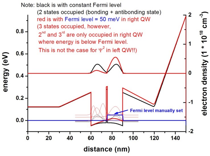
a) constant Fermi level at 0 eV:
The two quantum wells are nearly symmetric having one
bonding and one antibonding state that contribute to the density.
a) constant Fermi level at 0 eV and a constant
Fermi level of 50 meV in the right quantum well:
Now, the self-consistent solution of the Schrödinger-Poisson
equation leads to an asymmetric conduction band
profile.
The density of the right quantum well is now larger.
There are further options to manipulate the Fermi levels, see
Fermi level.
Importing arbitrary generation rate profile
import-generation = yes


= no
Flag whether to import the generation rate profile (yes
or no).
filename-generation =
read_in_generation_rate.dat
Filename of data file containing the data of the generation rate G(x,y,z) has to be present if
import-generation = yes.
   1D:  coordinate_x
	G(x)

     2D:  coordinate_x  coordinate_y
	G(x,y)

     3D:  coordinate_x  coordinate_y  coordinate_z
	G(x,y,z)
The units for coordinate_i are [nm]. The units of
the generation rate are 1018 [cm-3 s-1].
(For an example input file, please see the GaAs solar cell example.)
Importing arbitrary strain data
The flag whether to import strain has to be
specified via the keyword $simulation-flow-control.
strain-calculation = import-strain-simulation-coordinate-system
strain-calculation = import-strain-crystal-coordinate-system
Note: The strain tensor has to be given either with respect to the simulation
coordinate system or crystal coordinate
system. Please have a look here for details.
filename-strain = strain_data.dat
Filename of data file containing strain data has to be present if
strain-calculation = import-strain-....
The strain to be read in must not be given in Voigt notation, it must be given
in ordinary tensor notation and must refer to the simulation or crystal coordinate system.
   1D:  coordinate_x                              exx  eyy
  ezz  exy  exz  eyz

     2D:  coordinate_x  coordinate_y                exx  eyy
  ezz  exy  exz  eyz

     3D:  coordinate_x  coordinate_y  coordinate_z  exx  eyy
  ezz  exy  exz  eyz
The units for coordinate_i are [nm]. The strain tensor
units are dimensionless [].
Note: The eij components refer to shear strain
and not to "engineer shear strain".
Shear strain is the average of two strain tensor components, i.e.
eij = 1/2 (dui/dxj + duj/dxi)
whereas engineering shear strain is defined as the total shear strain
eij = dui/dxj + duj/dxi.
|