alloy-function
Specification of ternary alloy profile
For ternary materials, a name of an alloy function must be provided in the
material specification.
The parameters for various built-in functions which
generate the alloy profile have to be specified within the present keyword
$alloy-function.
Note: Can be used with an alloy
concentration sweep where the xalloy concentration is varied
stepwise.
!-----------------------------------------------------!

$alloy-function
optional !

 material-number              integer
required !

 function-name
 character
required !


!

 xalloy
 double
optional !

 xalloy-minimum
 double
optional !
for gaussian, one-minus-gaussian,
biparabolic
 xalloy-maximum
 double
optional ! gaussian, one-minus-gaussian
 gauss-center
double_array optional ! gaussian, one-minus-gaussian
 gauss-width
double_array optional ! gaussian, one-minus-gaussian
 rotation-angles              double_array
optional ! gaussian, one-minus-gaussian
! (probably some more later on)
 gauss-plane
 integer_array  optional !
gaussian-2d, e.g. (0,1,1)
 gauss-dir
 integer_array  optional !
gaussian-1d, e.g. (0,1,0)
 orientation
integer_array optional ! linear, e.g. (0,1,0);
!bilinear, e.g. (1,1,0)
 xalloy-from-to
 double_array   optional !
for linear
vary-from-pos-to-pos double_array
optional ! for linear
xalloy-at-corners double_array
optional ! for bilinear (four values)
 position-corners             double_array
optional ! bilinear (eight values, i.e. four
!
 Fermi-function-lambda
 double
optional !
 origin
 double_array
optional !
 trumpet-parameters           double_array
optional !
 onion-parameters             double_array
optional !
for onion shape alloy profile
C1,C2,C3,alpha in quantum dots
!

 filename-alloy-profile
character
optional !
for importing an alloy function
!

 function
character
optional !
!

 alloy-sweep-active
character
optional !
 alloy-sweep-step-size
double
optional !
 alloy-sweep-number-of-steps  integer
optional !
$end_alloy-function
optional
!

!-----------------------------------------------------!
material-number = integer
The material number of a ternary alloy material as given in the input file to
which this function applies to.
function-name = constant
! 1D,2D,3D


= linear
! 1D,2D,3D


= parabolic
! 1D,2D,3D
 =
biparabolic
!    2D,3D


 =
triparabolic
!       3D


= Fermi-function
! 1D,2D,3D
= gaussian-1d
! 1D,2D,3D

              =
gaussian-2d
!    2D,3D


= gaussian-3d
!       3D

              =
one-m-gaussian-1d                  ! 1D,2D,3D

              =
one-m-gaussian-2d                  !
2D,3D

              = one-m-gaussian-3d
!       3D

              =
bilinear
!    2D,3D

              = inv-triangle                       !       3D
= trumpet
    !       3D
= onion
    !       3D
= import-alloy-profile               ! 1D,2D,3D


= alloy-profile-defined-by-function  ! 1D,2D,3D


= xy-gaussian-3d
  !
The
'xy-...' functions are probably needed for quaternaries.
= xy-gaussian-2d
   !


= xy-gaussian-1d
   !


= xy-one-m-gaussian-3d
 !


= xy-one-m-gaussian-2d
 !


= xy-one-m-gaussian-1d
 !


= xy-constant
  !


= xy-linear
  !


= xy-bilinear
 !
String is one of the predefined function names. Depending on the dimension of
the simulation, various functions are available. The function names and
their parameters are described in the following.
The x values of the alloys (Si1-xGex, AlxGa1-xAs,
...) are written out automatically and can be visualized: alloy_grid1D.dat
One-dimensional simulations
function-name = constant
xalloy        = x
!

xalloy        =
0.2        ! e.g. Al(x)Ga(1-x)As,
Al0.2Ga0.8As
for constant alloy concentration
the constant x in AxB1-xC
0 <= x <= 1
Note: Can be used with an alloy
concentration sweep where the xalloy concentration is varied
stepwise.
function-name        =
linear


orientation          =
i j k
(0 0 1) or (0 1 0) or (1 0 0) the alloy
concentration varies along the selected simulation axis
vary-from-pos-to-pos = pos1 pos2
!
in units of [nm]
Alloy concentration varies from pos1 to pos2
with respect to selected
axis. pos1 < pos2
Example: vary-from-pos-to-pos = 75.0 125.0
xalloy-from-to       = x1 x2

x1
= alloy concentration at
pos1, x2 = alloy
concentration at pos2,
Outside the values (pos1, pos2) it is constant as specified by the boundary values
(x1, x2).
Example: xalloy-from-to = 0.2 0.8
|
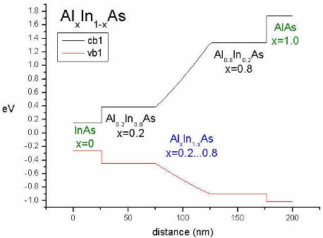 |
This conduction and valence band plot was generated by
specifying:
Material 1 (cluster-numbers = 1):
0 nm - 25 nm
Material 2 (cluster-numbers = 2):
25 nm - 175 nm
Material 3 (cluster-numbers = 3):
175 nm - 200 nm
but
vary-from-pos-to-pos:
75 nm -
150 nm (pos1
- pos2)
---> Outside the values pos1 and
pos2
the boundary values x1=0.2 and
x2=0.8 are taken
(between 25-75 and 125-175).
    $material


 material-number = 1

 material-name   = Al(x)In(1-x)As

 cluster-numbers = 1

 alloy-function  = constant


 material-number = 2

 material-name   = Al(x)In(1-x)As

 cluster-numbers = 2

 alloy-function  = linear


 material-number = 3

 material-name   = Al(x)In(1-x)As

 cluster-numbers = 3

 alloy-function  = constant


    $end_material
    $alloy-function


 material-number      = 1

 function-name        =
    constant

 xalloy
    = 0.0           ! -> InAs


 material-number      = 2

 function-name        =
    linear

 orientation
    = 0 0 1

 vary-from-pos-to-pos = 75.0 125.0

 xalloy-from-to       =
    0.2 0.8       ! -> from: Al0.2In0.8As

                                          ! -> to:   Al0.8In0.2As

 material-number      = 3

 function-name        =
    constant

 xalloy
    = 1.0
    ! -> AlAs


    $end_alloy-function
|
function-name        =
parabolic


orientation          =
i j k
(0 0 1) or (0 1 0) or (1 0 0) the alloy
concentration varies along the selected simulation axis
vary-from-pos-to-pos = pos1 pos2
!
in units of [nm]
Alloy concentration varies from pos1 to pos2
with respect to selected
axis. pos1 < pos2
Example: vary-from-pos-to-pos = 75.0 125.0
xalloy-from-to       = xmin xmax   !
xmin < xmax
and
xmin > xmax are allowed.
xminxmax = alloy
concentration at positions pos1
and pos2.
Outside the values (pos1, pos2) it is constant as specified by the boundary values
(xmax).
Example: xalloy-from-to = 0.2 0.8
Note: The origin of the parabola is set to: (pos2
-
pos1) / 2.
For more details on the parabolic alloy profile, have a look in the
Parabolic quantum well
tutorial.
function-name         =
Fermi-function   !
This can be used to model interdiffusion of atoms at interfaces.
orientation           =
i j k
0 0 1) or (0 1 0) or (1 0 0) the alloy
concentration varies along the selected simulation axis
vary-from-pos-to-pos  = pos1 pos2
!
in units of [nm]
Alloy concentration varies from pos1 to pos2
with respect to selected
axis. pos1 < pos2
Example: vary-from-pos-to-pos = 75.0 125.0
xalloy-from-to        = xmin xmax   !
xmin < xmax
and
xmin > xmax are allowed.
xmin
pos1,
xmax = alloy concentration at position
pos2.
Outside the values (pos1, pos2) it is constant as specified by the boundary values
(xmin or xmax,
respectively).
Example: xalloy-from-to = 0.2 0.8
origin =
pos_center !
center coordinate of the Fermi function in units of [nm] (pos1 <
pos_center < pos2)
Note: Even in 2D or 3D only one coordinate is expected (i.e. the one that
corresponds to the digit 1 in
orientation = i j k).
Fermi-function-lambda = 0.25 !
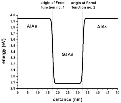
The quantum well is not assumed to be rectangular (as it is usually the
case). It has a Fermi function like alloy profile (i.e. AlxGa1-xAs
where x varies like a Fermi function) at the material interfaces (one Fermi
function at the left, and one at the right material interface).
The origin of the left Fermi function is at 17.5 nm, the origin of the right
Fermi function is at 32.5 nm.
The steepness parameter has been set to 0.25 (Fermi-function-lambda =
0.25).
If you want to obtain the input file for the Fermi function like quantum well (1DFermiFunctionLikeAlloyProfile.in),
please submit a support ticket.
function-name  = gaussian-1d


gauss-dir      = i j k
(0 0 1) or (0 1 0) or (1 0 0) the alloy
concentration varies along the selected simulation axis
gauss-center   = pos1

pos1
= position of Gauss center (position of xmax) along direction
specified by gauss-dir
gauss-width    = sigma

gauss-width
is usually called sigma in the formula of the Gaussian
distribution function.
xalloy-minimum = xmin
minimum value of alloy concentration
xalloy-maximum = xmax
maximum value of alloy concentration
function-name = one-m-gaussian-1d
gauss-dir = i j k
(0 0 1) or (0 1 0) or (1 0 0) the alloy
concentration varies along the selected simulation axis
gauss-center = pos1
pos1 = position of gauss center (position of
xmin) along direction
specified by gauss-dir
gauss-width = sigma
For the meaning of sigma
have a look at the
10 DM
banknote of the German "Deutsche Mark" or any mathematical textbook.
xalloy-minimum = xmin
minimum value of alloy concentration
xalloy-maximum = xmax
maximum value of alloy concentration
Two-dimensional simulations
All of the one dimensional functions can be used to generate profiles which
are constant along one coordinate axis. Additionally we have
function-name   = gaussian-2d

gauss-plane     = i j k
!
specifies the plane in which the alloy concentration varies, e.g. 0 1 1
gauss-center = pos1 pos2 ! specifies the
coordinates of the gauss maximum with
! respect to the coordinate plane selected
gauss-width = sig1 sig2 !
! gauss-plane
xalloy-minimum = xmin !
xalloy-maximum = xmax !
rotation-angles = angle !
! gauss-plane in [rad]
function-name   = one-m-gaussian-2d

gauss-plane     = i j k
!
specifies the plane in which the alloy concentration varies, e.g. 0 1 1
gauss-center = pos1 pos2
! specifies the coordinates of the gauss minimum
! with respect to the coordinate plane selected
gauss-width     = sig1 sig2
!
! selected by gauss-plane
xalloy-minimum  = xmin
!
xalloy-maximum  = xmax
!
rotation-angles = angle
!
! gauss-plane in [rad]
function-name     = bilinear
!

orientation       = i j k
!
variation of alloy concentration in this coordinate plane, e.g. 1 0 1
position-corners = pos1 ... pos8 ! four pairs of coordinates for
corners of a rectangle in plane selected by orientation
x1,y1
(1)
x2,y1
(2)
x2,y2
(3)
x1,y2
(4)
Same names indicate equal numbers!
x,y pairs refer to the plane in which the
alloy concentration varies.
 -----------------------------------

|x1,y2
(4)
x2,y2
(3)|
|
|
|
|
|
|
|x1,y1
(1)
x2,y1
(2)|
-----------------------------------
xalloy-at-corners = x1 ... x4 ! the alloy
concentration at the corners defined above
function-name     = biparabolic
!

orientation       = i j k
!
variation of alloy concentration in this coordinate plane, e.g. 1 0 1
position-corners = pos1 ... pos8 ! four pairs of coordinates for
corners of a rectangle in plane selected by orientation
x1,y1
(1)
x2,y1
(2)
x2,y2
(3)
x1,y2
(4)
Same names indicate equal numbers!
x,y pairs refer to the plane in which the
alloy concentration varies.
 -----------------------------------

|x1,y2
(4)
x2,y2
(3)|
|
|
|
|
|
|
|x1,y1
(1)
x2,y1
(2)|
-----------------------------------
xalloy-at-corners = x1 ... x4 ! the alloy
concentration at the corners defined above
xalloy-minimum    = xmin
!
minimum value of alloy concentration in the center of the rectangle
For more details on the biparabolic alloy profile, have a look in the
tutorial: Fock-Darwin states of a 2D parabolic potential in a magnetic field.
Three-dimensional simulations
All of the one- and two-dimensional functions can be used to generate alloy
profiles. Additionally we have:
function-name     = triparabolic
!
(can be used for quantum dots for example)
position-corners = pos1 ... pos16 !
position-corners  = 10.0 10.0 10.0
! (x1,y1,z1), corner (1)


20.0 10.0 10.0 !
(x2,y1,z1), corner (2)


20.0 20.0 10.0 !
(x2,y2,z1), corner (3)


10.0 20.0 10.0 ! (x1,y2,z1), corner (4)


10.0 10.0 20.0 ! (x1,y1,z2), corner (5)


20.0 10.0 20.0 !
(x2,y1,z2), corner (6)


20.0 20.0 20.0 ! (x2,y2,z2), corner (7)


10.0 20.0 20.0 !
(x1,y2,z2), corner (8)


xalloy-at-corners = x1 ... x8     !
the alloy
concentration at the corners defined above (at present, all values must be
equal)
xalloy-minimum    = xmin
!
minimum value of alloy concentration in the center of the cuboid
For more details on the triparabolic alloy profile, have a look at the
biparabolic alloy profile in the tutorial:
Fock-Darwin states of a 2D parabolic potential in a magnetic field
or submit a support ticket
for an example input file.
function-name   = gaussian-3d    !

gauss-center    = pos1
pos2 pos3 !
specifies the
coordinates of the gauss maximum
! with respect to the coordinate plane selected
gauss-width     = sig1
sig2 sig3 !
! gauss-plane
xalloy-minimum  = xmin
!
xalloy-maximum  = xmax
!
rotation-angles = angle1 angle2 !
! gauss-plane in [rad]
function-name   = one-m-gaussian-3d !

gauss-center    = pos1
pos2 pos3    !
specifies the coordinates of the gauss minimum
! with respect to the coordinate plane selected
gauss-width     = sig1
sig2 sig3    !
! by gauss-plane
xalloy-minimum  = xmin
!
xalloy-maximum  = xmax
!
rotation-angles = ang1 ang2
ang3 ! [rad]
Quantum dots
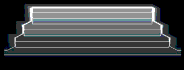
For a quantum dot, one can take e.g. four different alloy profiles:
origin
= 20.0  20.0  11.0  !
origin
of apex located at point (x,y,z)=(20 nm, 20 nm, 11 nm)
for inverse triangular and trumpet profile in quantum dots (e.g.
InGaAs)
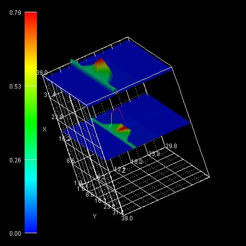
alloy-function = inv-triangle
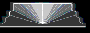
This formula considers an
additional lateral variation of the indium content.
      x = xmax - ( xmax - xmin
) cos2(phi)
where phi is the angle to the
center axis. The formula is based on the model proposed by Tersoff (N. Liu et
al., PRL 84, 334 (2000)).
with high indium content for small
angles as indicated by the light regions in the figure shown below.
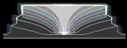
alloy-function = trumpet
trumpet-parameters = C1
  C2   0.3   0.8  !
   C1   C2
  C3  alpha
for trumpet shape alloy profile
C1,
C2, C3,
alpha in quantum dots.
The minimum and maximum indium concentrations are given by
xmax
  = 1 - C1
xmin
  = 1 - C2
The parameters C3 and
alpha can be used to vary the shape of the
alloy profile while keeping the average indium content fixed. (M. Sabathil used
C3 = 0.3 and
alpha = 0.8 for InGaAs dots) .
The symmetry center is set by the specifier
origin.
Note: So far it only works for the growth
direction being the z axis.
The indium concentration is given by this formula:
rho = SQRT(x2 + y2)
    f(x,y,z) = 1 - [
	C2 + (C1 -
	C2) exp [ ( - rho  exp (- 2
	z C3) ) / {alpha}
	] ] =


             =  xmin
  	+ ( xmax - xmin) exp [ ( - rho
	exp (- 2 z C3) ) / {alpha}
	]
The formula is based on the more refined model proposed by Migliorato
(M.A. Migliorato et al., PRB 65, 115316 (2002)).
trumpet.
Example
- Quantum dot with inverse triangular alloy shape ("inverted pyramid")
$material
  !

 ...

 material-number = 5
  !

 material-name   = In(x)Ga(1-x)As
  !
InGaAs quantum dot
 cluster-numbers = 5
  !

 alloy-function  = inv-triangle
  !

 ...

  $end_material
  !


  $alloy-function
  !

 ...

 material-number = 5
  !

 function-name   = inv-triangle
  !

 origin          =
20.0 20.0 11.0 ! (x,y,z)=(20,20,11) (top of inverted
pyramid)
 xalloy-from-to  = 0.28
0.80 ! 0.28:
In0.28Ga0.72As)
! 0.80: In0.80Ga0.20As)
 ...

  $end_alloy-function
Red (80 % In): In0.80Ga0.20As
Onion profile for quantum dots
Thanks to T. Fromherz, University of Linz, for implementing the function
onion.
alloy-function = onion
onion-parameters = 0.2    C2
	C3   0.0    !
   C1   C2
  C3  alpha
for onion shape alloy profile
C1,
C2, C3,
alpha in quantum dots.
C1: background alloy
concentration
in units of []
C2:
vertical alloy concentration variation in units of [nm-0.5]
C3:
lateral alloy concentration variation in units of [nm-2]
(alpha: currently not used but
this dummy parameter has to be present)
The alloy concentration is given by this formula where x,y,z
refer to the simulation coordinate system in units of [nm]:
rho = SQRT(x2 + y2)
alloyc = C1 +
		C2 * SQRT(z) +
		C3 * rho2
The symmetry center is set by the specifier
origin.
Note: So far it only works for the growth
direction being the z axis.
Example
- Quantum dot with onion alloy shape
(...has to be added)
User-defined alloy function (new)
Using the alloy function alloy-profile-defined-by-function, one can define an
arbitrary function n(x,y,z) for the alloy profile.
The variables x, y, z refer to the grid point coordinates of the simulation area
in units of [nm].
Example: A parabolic alloy profile.
$material

 ...

 alloy-function =
alloy-profile-defined-by-function

     ...

    $alloy-function

 ...

 %K = 0.02

     function-name  =
alloy-profile-defined-by-function

 function       = " 1/2
* %K * (z-15)^2 "
! alloy(x,y,z) = ...
In this example, the parabolic alloy function
profile is shifted by 15 nm along the z axis.
The following operators and functions are supported:
+ , - ,
	* , / , ^

	abs , exp , sqrt
	, log , log10
	, sin , cos
	, tan , sinh ,
	cosh , tanh , asin
	, acos , atan
If the function leads to a value smaller than 0.0, then 0.0 is taken for the
alloy concentration.
If the function leads to a value larger than 1.0, then 1.0 is taken for the
alloy concentration.
Reading in alloy profiles from a file
alloy-function = import-alloy-profile
filename-alloy-profile = "D:\nextnano
simulations\alloy_function.dat"
                       =
 D:\nextnano_simulations\alloy_function.dat
alloy profile filename to be read in (e.g. experimental values). The string can
include a folder name.
The ASCII file must contain 2 (1D), 3 (2D) or 4 (3D) columns in each line:
1D:
x coordinate [nm]
alloy concentration

...
...
2D:
x coordinate [nm]    y coordinate [nm]
alloy concentration

...
...
...
3D:
x coordinate [nm]    y coordinate [nm]   z coordinate
[nm]
alloy concentration

...
...
...
...
It must hold: 0 <= alloy concentration <= 1
The first line of this ASCII file can contain an optional header line
with column descriptors.
If you want to obtain input files that show how to import an alloy profile
from a file please submit a support ticket.
1DFermiFunctionLikeAlloyProfile_read_in_alloy_profile.in
2D_InGaAs_GaAs_QW_arbitrary_alloy_profile_xz_rect.in
It is possible to sweep over the alloy concentration, i.e. to vary the
alloy concentration stepwise.
In each alloy sweep step, the specifier xalloy (constant
alloy function) is
increased by alloy-sweep-step-size.
The output is labelled by ..._ind000.dat, ..._ind001.dat,
... for each alloy sweep step.
 alloy-sweep-active           =
yes       !
to
switch on alloy sweep
= no !
 alloy-sweep-step-size        =
0.05
!
increase alloy concentration in each step by 0.05
!
 alloy-sweep-number-of-steps  = 5
!
Restrictions:
- Voltage sweeps ($voltage-sweep)
and other sweeps cannot be combined with alloy sweeps at present.
- Only one alloy sweep is allowed at present.
For code developers
If you want to add new alloy functions to the code, you will have to modify
these files:
database_nn3.in
==>
  $known-function-names
==> Simply add name of the new alloy function in an analogous
manner. This is trivial.input_parser / alloy /
allocate_alloy_structures.f90
==> Simply add name of the new alloy function in an analogous manner.
This is trivial.input_parser / alloy /
alloy_param_type.f90
==> Simply add new MODULE and variables of the new alloy function in an
analogous manner. This is easy.input_parser / read_profile_parameters /
read_alloy_data.f90
==> Simply add name of the new alloy function in an analogous manner.
This is trivial.input_parser / read_profile_parameters /
read_para_constant.f90 (Here: constant
alloy function)
==> input_parser / treat_profiles /
alloy.f90
==> Simply add name of the new alloy function in an analogous manner.
This is trivial.input_parser / treat_profiles /
constant.f90
==> Simply add the equations that calculate the alloy concentration (as
a function of grid points) of the new alloy function in an analogous manner.
That's it!
Don't forget to test your new alloy function thoroughly in 1D, 2D and 3D,
as well as for different orientations:
- 1D: growth along x, y or z
- 2D: (x,y) plane, (y,z) plane, (x,z)
plane)
- 3D: is okay (only one orientation is
possible)
|