|
| |
nextnano3 - Tutorial
next generation 3D nano device simulator
3D Tutorial
Cleaved edge overgrowth quantum dots (CEO QDs)
Author:
Stefan Birner
If you want to obtain the input files that are used within this tutorial, please
check if you can find them in the installation directory.
If you cannot find them, please submit a
Support Ticket.
-> 3DTshapedQD_CEO_4nm_no_exciton.in - (The calculation
takes 13 minutes SYSTEM time and 38 minutes CPU time on a modern Quad-core CPU.)
 -> 3DTshapedQD_CEO_4nm.in

 -> 3DTshapedQD_CEO_5nm.in

 -> 3DTshapedQD_CEO_7nm.in

 -> 3DTshapedQD_CEO_9nm.in
Cleaved edge overgrowth quantum dots (CEO QDs)
- This tutorial is based on the paper of
M. Grundmann, D. Bimberg
Formation of quantum dots in twofold cleaved edge
overgrowth
Phys. Rev. B 55 (7), 4054 (1997).
The purpose is to benchmark the nextnano³ code to their numerical
calculations.
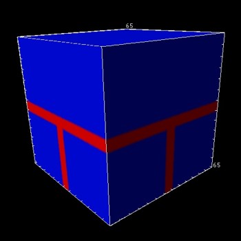
- We study T-shaped cleaved edge overgrowth quantum dots (CEO QDs) that consist of three
perpendicularly oriented quantum wells that are placed inside a 65 nm x 65 nm x
65 nm cuboid of Al0.35Ga0.65As.
If the width of all three
GaAs quantum wells is 5 nm, the structure looks as follows:
|
 |
 |
 |
| |
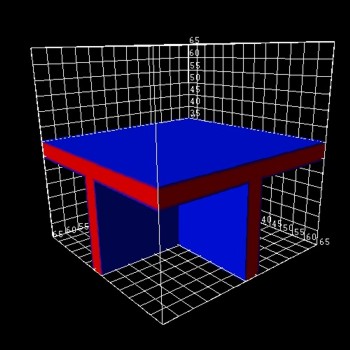
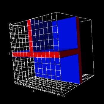
(only the three GaAs QWs are shown) |
(only the three GaAs QWs are shown) |
| |
|
|
- The axes are oriented the following way:
  $domain-coordinates

   ...

   hkl-x-direction-zb = 0  0  1  !
along the
[001] direction in the crystal coordinate system (1st
growth direction, i.e. 1st QW)
hkl-y-direction-zb = 1 -1 0 !
!hkl-z-direction-zb = 1 1 0 !
- The intersection of the three T-shaped quantum wires (QWRs) forms the
quantum dot (i.e. in the middle of the structure).
- In accordance to the above cited paper, we solve the single-band
Schrödinger equation using isotropic effective masses for the electrons and
for the heavy holes.
We use Neumann boundary conditions for the Schrödinger equation.
The Schrödinger matrix has dimension N = Nx * Ny * Nz
= 65 * 65 * 65 = 274625.
(65 grid points in each direction, i.e. a 1 nm grid spacing.)
- From the calculated single-particle electron and heavy hole ground states,
we calculate the exciton binding energy within the Hartree approximation
(Coulomb interaction).
The algorithm is as follows:
1) Solve Schrödinger equation for the
single-particle energies and wave functions of the electron
(empty dot).
2) Solve Schrödinger equation for the
single-particle energies and wave functions of the heavy hole
(empty dot).
a) Solve Poisson equation for the electrostatic potential of the
electron ground state density.
b) Solve Schrödinger equation for the
single-particle energies and wave functions of the heavy hole
including electrostatic potential of electron.
c) Solve Poisson equation for the electrostatic potential of the
heavy hole ground state density.
d) Solve Schrödinger equation for the
single-particle energies and wave functions of the electron
including electrostatic potential of electron.
Iterate a), b), c), d) until convergence of exciton energy. (It usually
converges within 4-5 iterations.)
The total number of iterations and the residual can be specified in the input
file:
  $numeric-control

   ...

   coulomb-matrix-element
  = yes

   calculate-exciton
  = yes

   exciton-iterations
  = 7     !
number of
iterations for exciton convergence
   exciton-residual
  = 1d-5  !
   exciton-electron-state-number
  = 1     !
  1
   exciton-hole-state-number
  = 1     !
  1
   number-of-electron-states-for-exciton = 1
  ! 1
   number-of-hole-states-for-exciton     =
  1     !
  1
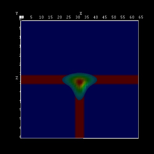
- The following figure shows the square of the
(excitonic) electron wave function (70 % of psi2).
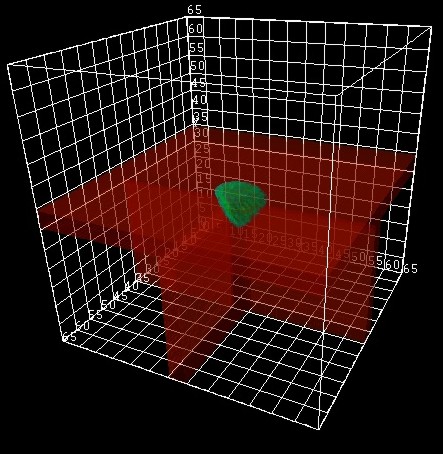
- The following figure shows the square of the (excitonic) electron
wave function (slice inside the third quantum well plane, i.e. the slice
is only through GaAs).
Note that the slice of the material grid is below the third quantum well plane
(slice through Al0.35Ga0.65As/GaAs).
The x axis is along the [001] direction in the crystal coordinate
system (1st growth direction, i.e. 1st QW).
- The calculated exciton binding energies for CEO QDs of lengths 4 nm, 5 nm,
7 nm and 9 nm are shown in the following figure.
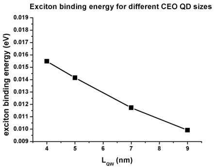
The results are in reasonable agreement with Grundmann's paper although our
values are about 2 meV smaller.
We solved the Schrödinger and Poisson equations on a homogenous 65 nm x 65 nm
x 65 nm grid using a grid resolution of 1 nm (which is a rather coarse grid),
i.e. the total number of grid points is 66 x 66 x 66 = 287496.
|