nextnano³ - Tutorial

next generation 3D nano device simulator

2D Tutorial

Single-band ('effective-mass') is a special case of 8-band k.p ('8x8kp') if the electrons are decoupled from the holes

Author: Stefan Birner

If you want to obtain the input file that is used within this tutorial, please submit a support ticket.
-> effective_mass_vs_8x8kp_sg_2D.in
-> effective_mass_vs_8x8kp_kp_2D.in
-> effective_mass_vs_8x8kp_density_sg_2D.in
-> effective_mass_vs_8x8kp_density_kp_2D.in
-> effective_mass_vs_8x8kp_same_mass_sg_2D.in
-> effective_mass_vs_8x8kp_same_mass_kp_2D.in

1) Single-band ('effective-mass') is a special case of 8-band k.p ('8x8kp') if the electrons are decoupled from the holes

Input file -> 2Deffective_mass_vs_8x8kp.in

Note: This tutorial is identical to the 1D tutorial "Single-band ('effective-mass') is a special case of 8-band k.p ('8x8kp') if the electrons are decoupled from the holes".
The only difference is that it is 2D.

In 1D, the simulated structure is 45 nm long.
In 2D, the simulated structure is 45 nm long and 5 nm wide (y axis). Along the y axis, we apply periodic boundary conditions to the Schrödinger equation, so that the structure is effectively infinitely long.

Results

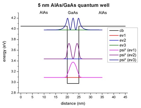
• The following figure shows the conduction band profile and the three lowest (confined) eigenstates for k=0 including their charge densities (wave function Psi²) for a 5 nm AlAs/GaAs quantum well.
  
  1D plot of the 1D tutorial:
  
  
  2D plot of the 2D tutorial:
  
  
  
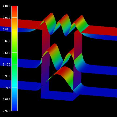
  The scale on the left corresponds to the conduction band edge energies of the barrier (4.049 eV) and the well (2.979 eV).

We want to stress that we solved a two-dimensional Schrödinger equation in 2D and not only a one-dimensional one as in 1D.

The calculated eigenvalues can be found in the files
1D: Schroedinger_1band/ev1D_cb001_qc001_sg001_deg001_dir   _Kx001_Ky001_Kz001.dat
2D: Schroedinger_1band/ev2D_cb001_qc001_sg001_deg001_dirper_Kx001_Ky001_Kz001.dat
                                              dirichlet   boundary condition along x
                                                 periodic boundary condition along y


Both, 1D and 2D, and both, effective-mass and 8x8kp lead to exactly the same eigenvalues. Also the squared wave functions (Psi²) are identical. The squared wave functions are normalized in units of [1/nm²] so that they integrate to 1.0 if the integration interval is over the area from 10 nm to 35 nm along the x axis and from 0 nm to 5 nm along the y axis. (The rectangle of the quantum cluster extends from 10 nm to 35 nm along x and from 0 nm to 5 nm along y.) Note that the probabilities Psi² are shifted by the corresponding eigenvalues so that they fit nicely into the graph. Here, the color dark blue corresponds to zero probability of Psi².

Note:
Single-band
- schroedinger-masses-anisotropic = yes: Periodic boundary conditions not implemented yet.
- schroedinger-masses-anisotropic = box: Periodic boundary conditions implemented but do not work if the quantum cluster coincides with the whole device volume:
  'Error get_sg_material_parameters: i_material out of range.'
  Thus the quantum region has to be reduced to a length of 4 nm, i.e. from 0 to 4 nm (if the gridding is in steps of 1 nm) because 'box'
  assumes that there is an additional grid point between 4 nm and 0 nm when applying periodic boundary conditions.
8-band k.p
- schroedinger-kp-discretization = finite-differences: Periodic boundary conditions not implemented yet.
- schroedinger-kp-discretization = box-integration: Periodic boundary conditions implemented but do not work if the quantum cluster coincides with the whole device volume:
  'Error get_8x8_kp_zb_parameters: Number of point out of range.'
  Thus the quantum region has to be reduced to a length of 4 nm, i.e. from 0 to 4 nm (if the gridding is in steps of 1 nm) because 'box-integration'
  assumes that there is an additional grid point between 4 nm and 0 nm when applying periodic boundary conditions.

2) Calculating the quantum mechanical density within the single-band approximation and 8-band k.p self-consistently

Input file -> 2Deffective_mass_vs_8x8kp_density.in

Our input file contains a similar 5 nm quantum well but instead of AlAs we take Al_0.2Ga_0.8As as the barrier material. However, this time we include some n-type doping with a concentration of 1*10¹⁷ cm^-3. Only the AlGaAs region between 35 and 40 nm (along the x axis) is doped. The donor atom has a donor level of 0.007 eV below the conduction band.

We use flow-scheme = 2, i.e.
- we solve the Poisson equation including doping to obtain the electrostatic potential
- we use this electrostatic potential to solve Schrödinger's equation effective-mass (single-band) approximation
- we calculate the electron density (including quantum mechanical density) that enters the Poisson equation
- we solve the Poisson and Schrödinger equation self-consistently

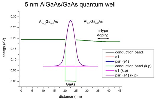
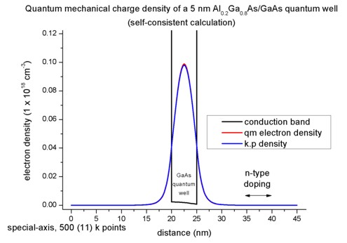
The following figure shows the conduction band profile and the lowest eigestate as well as its probability amplitude. The chemical potential (i.e. the Fermi level) is not shown in the figure. It is equal to 0 eV. There are no further eigenstates that are confined inside the well. (The figure also shows the k.p results which are identical.)

1D plot of the 1D tutorial:

2D plot of the 2D tutorial:



The scale on the left corresponds to the conduction band edge energies of the barrier and the well in units of [eV].

Note: In our example we take into account only the first quantized eigenstate. Usually one has to sum over all (occupied) eigenstates to calculate the quantum mechanical density.

The three-dimensional electron density of this 2D quantum structure (homogeneous along the z direction) can be calculated in the single-band effective-mass approximation (i.e. parabolic and isotropic bands) as follows:

1D: n(x) = g m_||,av k_BT / (2 pi h_bar²) |Psi₁(x)|² ln(1 + exp( (E_F(x) - E₁)/ (k_BT) ) )
Note the squared wave function |Psi₁|² must be normalized over the length of the quantum cluster, i.e. the units are 1/m.

2D: n(x,y) = 1/2 g [ m_z,av k_BT / (2 pi h_bar²) ]^1/2 |Psi₁(x,y)|² F_-1/2[ (E_F(x,y) - E₁)/ (k_BT) ]
Note the squared wave function |Psi₁|² must be normalized over the area of the quantum cluster, i.e. the units are 1/m².

(For 1D, confer also the corresponding equation in the overview section: "Purely quantum mechanical calculation of the density".)

• g is the degeneracy factor for both spin and valley degeneracy. In our case, the Gamma conduction band valley is not degenerate, so we have g = 2 to account for spin degeneracy.
• Usually m_z depends on the grid point (x,y), so we should have written m_z(x,y) instead of m_z,av. However, this leads to discontinuities in the quantum charge density as m_z(x,y) is discontinuous at material interfaces. A possible solution is to take an average of all m_z values in the quantum cluster weighted by the quantum charge density (Psi²). This leads to m_z,av = 0.0698246 (1D: m_||,av = 0.0698240)
• k_BT = 0.025852 eV (at 300 K)
• [m₀ k_BT / (2 pi h_bar²) ]^1/2 = 2.323704676 * 10⁸ 1/m
  Note that: [kg VAs / (J²s²)]^1/2 = [Ns²/m / (Js²)]^1/2 = [N/m / J]^1/2 = [1 / m²]^1/2 = [1/m]
• |Psi₁(x,y)|²: Probability amplitude of the wave function Psi₁ of the first eigenstate.
  The maximum value of |Psi₁(x=22.5 nm,y)|² is 0.04247 1/nm².
  This value, multiplied with the length of 5 nm (extension along the y direction) leads to 0.21235 1/nm and compares well with the 1D result of 0.21237 1/nm.
• E_F(x,y): Chemical potential (i.e. Fermi level). In our example it is equal to zero: E_F(x,y) = 0
• E₁ = 0.08366 eV: energy of the first quantized state (1D: E₁ = 0.07117 eV)

The Fermi-Dirac integral F_-1/2 (which includes the Gamma prefactor of the Fermi-Dirac integral) at position (x=22.5 nm,y) can be evaluated to: F_-1/2 [ (E_F(x,y) - E₁)/ (k_BT) ] = F_-1/2 [ -3.236173 ] = 0.0382551
 

We calculate the electron density for the grid point in the middle of the quantum well where the maximum of the probability amplitude occurs:

=> n(x = 22.5 nm,y) = 1/2 * 2 * (0.069824)^1/2 * 2.323704676*10⁸ 1/m * 0.04247 1/nm² * 0.0382551 = 9.9976 * 10²² 1/m³

This number divided by the three-dimensional number density (1*10²⁴) leads to 0.09976, i.e. the output is in units of 1 * 10¹⁸ cm^-3, thus the density equals 0.09976 * 10¹⁸ cm^-3 (1D result: 0.09893 * 10¹⁸ cm^-3)

This value is in agreement with the plot of the electron density. The density is dominated by the quantum mechanical contribution to the density. The classical contribution is negligible (i.e. only 0.00007 * 10¹⁸ cm^-3).

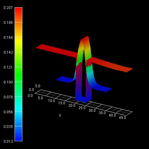
2D plot of the self-consistent electron charge density:



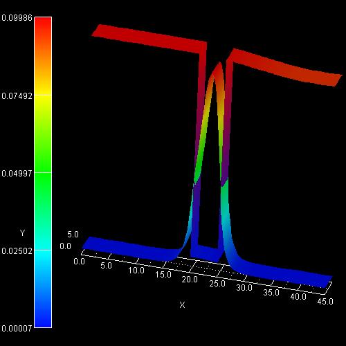
On the left side the figure shows the color map of the electron density (in units of 1 * 10¹⁸ cm^-3). Note that the color of the conduction band edge has nothing to do with it.

Compare to the 1D plot of the corresponding 1D tutorial:

3) Calculation of the quantum mechanical density from the k.p dispersion (no self-consistency)

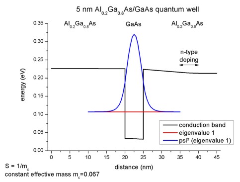
Input file -> 2Deffective_mass_vs_8x8kp_same_mass.in

To compare the k.p results with the effective-mass results it is easier to use for both materials the same conduction band effective mass. So even for Al_0.2Ga_0.8As we take the GaAs mass of 0.067 this time. The relevant 8-band k.p parameter S is then given by S = 1/m_e = 1/0.067 = 14.925.

We use the same doping as in 2) but this time we use flow-scheme = 3, i.e.
- we solve the Poisson equation including doping to obtain the electrostatic potential
- we use this electrostatic potential to solve Schrödinger's equation with both effective-mass (single-band) approximation and 8-band k.p. As expected the eigenvalues and wave functions coincide for these two cases. The energy of the lowest eigenstate is E₁ = 0.10707 eV (1D: E₁ = 0.10707).

Here is the 1D plot of the corresponding 1D tutorial (which is identical to the 2D case):

In order to calculate the k.p dispersion E(k_z), we have to solve the 8-band k.p Hamiltonian for different k_z (in-plane wavevector). As our electrons in the Hamiltonian are decoupled from the holes, we have the special case where the dispersion E(k_z) is parabolic. In 2D, the k.p dispersion is "isotropic" in any case as we only have one direction. Thus it is possible to plot (and calculate) the E(k_z) dispersion along a line only. In 1D, we had a 2D k space.

num-kp-parallel = 15
Our k space, i.e. k=k_z, contains 15 k points in the 1D Brillouin zone. Thus it is sufficient to integrate over the k points that are lying along the line of the 1D Brillouin zone.

The relevant data for the E(k_z) dispersion along the k_z direction is stored in the file: Schroedinger_kp/kpar2D_dispel_ev001.dat
It contains 15 k points and the corresponding eigenvalues.

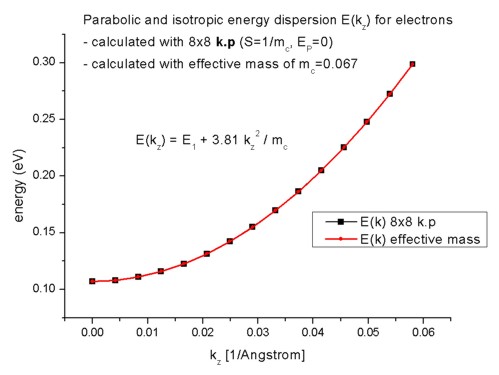
The parabolic dispersion is given by E(k_z) = E₁ + h_bar²/2m₀ k_z²/m_c
where h_bar²/2m₀ is given by 3.81 [eV Angstrom²] and the conduction band effective mass m_c is a dimensionless quantity here in this equation. k_z is given in [1/Angstrom]. E₁ is the energy of the lowest eigenstate E₁ = 0.10707 eV (1D: E₁ = 0.10707 eV). As expected, the dispersion for the effective-mass approximation agrees perfectly to the 8-band k.p case.

To calculate the k.p densities one has only one option to choose from so far for the integration over the 1D Brillouin zone:
method-of-brillouin-zone-integration = special-axis
                                     = gen-dos            (not implemented yet)
                                     = simple-integration (not applicable to a 2D simulation)

• special-axis uses a 1D integration along a line. The number of k_z points is taken from the input file (num-kp-parallel = 15).
• gen-dos calculates the density of states (DOS) and integrates over the DOS for obtaining the k.p density.

More details can be found in the glossary.

The following figure compares the quantum mechanical electron charge densities calculated with the effective-mass approximation and with k.p.

1D plot

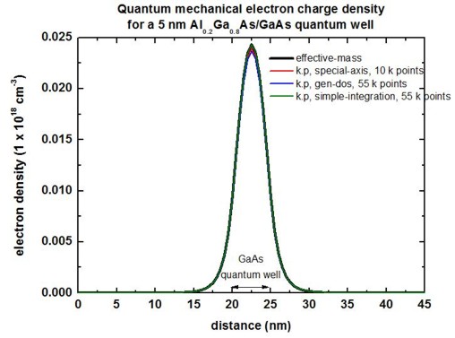
2D plot

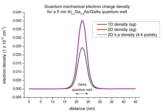
Here, the 2D k.p and single-band densities are in perfect agreement. Only 4 k_z points are necessary. However, the 2D density is different compared to the 1D case although the conduction bands, the eigenvalues, psi² and effective masses are in perfect agreement.

2D:

E₁ = 0.10707

The Fermi-Dirac integral F_-1/2 (which includes the Gamma prefactor of the Fermi-Dirac integral) at position (x=22.5 nm,y) can be evaluated to: F_-1/2 [ (E_F(x,y) - E₁)/ (k_BT) ] = F_-1/2 [ -4.141821 ] = 0.015717538

The maximum value of |Psi₁(x=22.5 nm,y)|² is 0.04265 1/nm².
This value, multiplied with the length of 5 nm (extension along the y direction) leads to 0.21325 1/nm and compares well with the 1D result of 0.21324 1/nm.

=> n(x = 22.5 nm,y) = 1/2 * 2 * (0.067)^1/2 * 2.323704676*10⁸ 1/m * 0.04265 1/nm² * 0.015717538 = 0.040320 * 10²⁴ 1/m³ = 0.04032 * 10¹⁸ 1/cm³

                                                                                                       If F_-1/2 were  0.094843, then the 2D result would be the same as the 1D one.

conduction band minimum: 0.03156 eV, conduction band maximum: 0.22592 eV

(k.p leads to the same density.)

1D:

E₁ = 0.10707

The logarithm at position x can be simplified to: ln(1 + exp(- 0.10707 / 0.025852)) = ln 1.0159 = 0.01577

Psi₁²(x = 22.5 nm) = 0.21324 1/nm

=> n(x = 22.5 nm) = 0.067 * 1.07992*10¹⁷ 1/m² * 0.21324 1/nm * 0.01577 = 2.43311 * 10²² 1/m³ =  0.02433 * 10¹⁸ 1/cm³

conduction band minimum: 0.03156 eV, conduction band maximum: 0.22592 eV

(For this tutorial example, we used k-range-determination-method = bulk-dispersion-analysis as here the automatic determination of k-range works well because the in-plane dispersion is the same as the bulk k.p dispersion. Note: The new input files use 'k-max-input' instead.)

Comments: It seems that for 2D and "box" (single-band) the results are slightly different compared to 2D and "box-integration" (8-band k.p).
This is a bit strange. The former results are a bit strange. This should be checked.