nextnano3 - Tutorial
next generation 3D nano device simulator
2D Tutorial
Hole wave functions in a quantum wire subjected to a magnetic field
Author:
Stefan Birner
If you want to obtain the input files that are used within this tutorial, please
check if you can find them in the installation directory.
If you cannot find them, please submit a
Support Ticket.
-> 2Dwire.in
(single-band approximation)
-> 2Dwire_magnetic.in
-> 2Dwire_6x6kp.in
-> 2Dwire_6x6kp_Burt.in
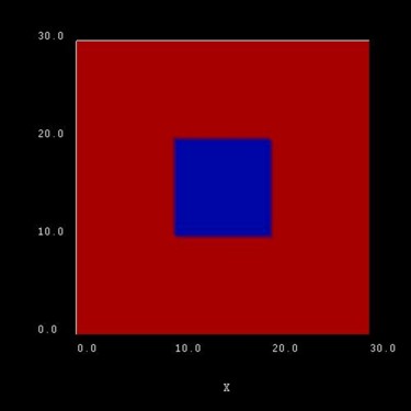
Quantum wire
Similar to the 1D confinement in a quantum well, it is possible to
confine electrons or holes in two dimensions, i.e. in a quantum wire.
The quantum wire consists of InAs (blue area) and is confined by GaAs barriers
(red area).
Its size is 10 nm x 10 nm whereas the whole simulation dimension is 30 nm x
30 nm.
 |
 |
|
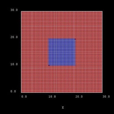
The blue area is the quantum wire which consists of InAs. The quantum wire
rectangle has the size 10 nm x 10 nm.
|
This picture shows a possible configuration of rectangular grid lines.
Here, the grid spacing is 0.5 nm, thus the quantum wire (blue area) consists
of 21 x 21 = 400 grid points.
|
Quantum cluster
Assumptions:
1) We apply Dirichlet boundary conditions to our quantum cluster (psi = 0
at the boundary).
2) The quantum cluster is defined only in the area of the quantum wire,
i.e. from 10 nm to 20 nm.
These two conditions lead to an infinite GaAs barrier and thus the
wave function is forced to be zero at the InAs quantum wire boundaries. Of
course, this is not a realistic assumption but we simplify the sample to make
the tutorial easier.
The energy levels and the wave functions of a rectangular quantum wire of length 10 nm
with infinite barriers can be calculated analytically.
We assume that the barriers at the QD boundaries are infinite. This way we
can compare our numerical calculations to analytical results.
The potential inside the quantum wire is assumed to be 0 eV.
As effective mass we take the isotropic heavy hole effective mass of InAs, i.e. mhh
= 0.41 m0.
valence-band-masses = 0.41d0 0.41d0 0.41d0 !
isotropic heavy hole
effective
...
A discussion of the analytical solution of the 2D Schrödinger equation of a
particle in a rectangle (i.e. quantum wire) with infinite barriers can be found in e.g.
Quantum Heterostructures (Microelectronics and Optoelectronics) by V.V.
Mitin, V.A. Kochelap and M.A. Stroscio.
The solution of the Schrödinger equation leads to the following eigenvalues
(where mhh is assumed to be negative):
En1,n2 = hbar2 pi2
/ 2mhh
( n12 / Lx2 + n22
/ Ly2) =
=
-9.1714667 * 10-19 eVm2 ( n12
/ Lx2 + n22 / Ly2) =
=
-0.0091714667 eV
( n12
+ n22 ) (if Lx
= Ly = 10 nm)
- En1,n2 is the heavy hole energy in the two
transverse directions, or the total heavy hole energy for kz = 0.
Note that the total heavy hole energy is given by Ehh = En1,n2
+ hbar2 kz2 / 2mhh
where kz is the wavevector along the z direction leading to a
one-dimensional E(kz) dispersion.
- n1, n22
are two discrete quantum numbers (because we have two
directions of quantization).
- Lx and Ly are the lengths along the x and y
directions. In our case, Lx = Ly =
10 nm.
Generally, the energy levels are not degenerate, i.e. all energies are
different.
However, some energy levels with different quantum numbers coincide, if
the lengths along two directions are identical (En1,n2 = En2,n1) or
if their ratios are integers. In our quadratic quantum wire, the two lengths are
identical.
Consequently, we expect the following degeneracies:
- E11 =
-0.018343 eV (ground state)
- E12 = E21 =
-0.045857 eV
- E22 =
-0.073372 eV
- E13 = E31 =
-0.091715 eV
- E23 = E32 =
-0.119229 eV
- E14 = E41 =
-0.155915 eV
- ...
- E18 = E81 = E47 = E74 =
-0.596145 eV (Here, the degeneracy is a coincidence.)
nextnano³ numerical results for a 10 nm quadratic quantum wire with 0.10 nm
grid spacing:
Output file name:
Schroedinger_1band/ev2D_vb001_qc001_sg001_deg001_dir_Kx001_Ky001_Kz001.dat
 num_ev: eigenvalue [eV]:

        (0.10 nm grid)


  1      0.018341
= E11
2 -0.045845
E12/E21
3 -0.045845
E12/E21
4 -0.073348
= E22
5 -0.091653
(two-fold degenerate) E13/E31
6 -0.091653
(two-fold degenerate) E13/E31
7 -0.119156
(two-fold degenerate) E23/E32
8 -0.119156 E23/E32
9 -0.155721
(two-fold degenerate) E14/E41
10 -0.155721
(two-fold degenerate) E14/E41
...
42 -0.593061
(four-fold degenerate) E18/E81 or E47/E74
43 -0.593061
(four-fold degenerate) E18/E81 or E47/E74
44 -0.594144
E18/E81 or E47/E74
45 -0.594144
(four-fold degenerate) E18/E81 or E47/E74
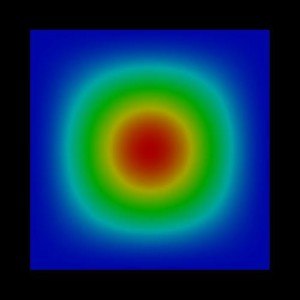
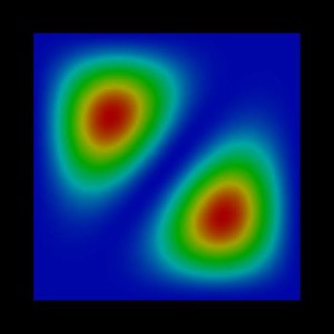
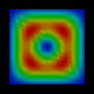
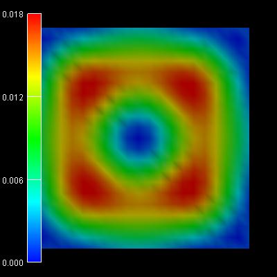
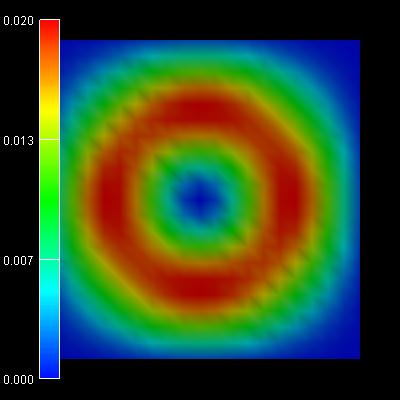
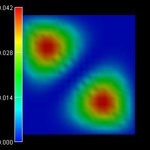
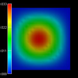
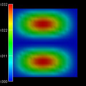
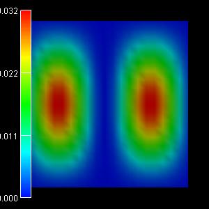
Hole wave functions - Single-band effective-mass approximation (infinite GaAs
barriers)
-> 2Dwire.in
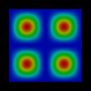
The following figures show the charge densities (Psi²; Psi = hole
wave function) of the four lowest energy confined hole eigenstates in an
infinitely deep 10 nm x 10 nm InAs quantum wire. Due to the symmetry of the quantum wire, the
second and the third eigenstate are degenerate.
 |
 |
|
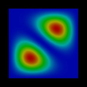
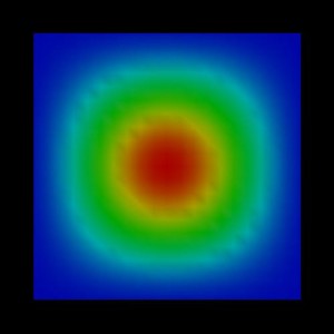
1st eigenstate: -0.0183 eV |
2nd eigenstate: -0.0458 eV |
 |
 |
|
3rd eigenstate: -0.0458 eV |
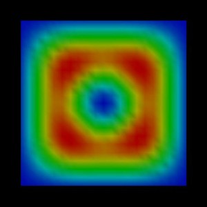
4th eigenstate: -0.0733 eV |
The heavy hole valence band edge energy of InAs is set to be located at 0 eV. The hole eigenvalues are:
schroedinger-masses-anisotropic =
yes |
= no |
= box |
1st eigenvalue =>
confinement energy: -0.018341 eV |
-0.018341 eV |
-0.018341 eV |
2nd eigenvalue =>
confinement energy: -0.045845 eV |
-0.045845 eV |
-0.045845 eV |
3rd eigenvalue =>
confinement energy: -0.045845 eV |
-0.045845 eV |
-0.045845 eV |
4th eigenvalue =>
confinement energy: -0.073348 eV |
-0.073348 eV |
-0.073348 eV |
Note that these wave functions were obtained by using a single-band
effective mass approximation for the holes. A more accurate and more
realistic treatmeant would have been to use 6-band k.p. Note that the wire
has been assumed to be unstrained (which is a rather unphysical situation) for
the purpose to make this tutorial easier to understand.
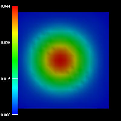
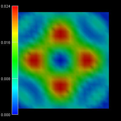
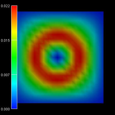
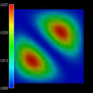
Magnetic field - single-band approximation (infinite GaAs barriers)
-> 2Dwire_magnetic.in
Here we use: schroedinger-masses-anisotropic =
yes ! 'yes', 'no',
'box'
We apply a magnetic field perpendicular to the (x,y) plane, i.e. along the
[001] direction.
$magnetic-field
magnetic-field-on =
yes
magnetic-field-strength = 1.0d0 ! 1
Tesla
magnetic-field-direction = 0 0 1 ! [001]
direction
$end_magnetic-field
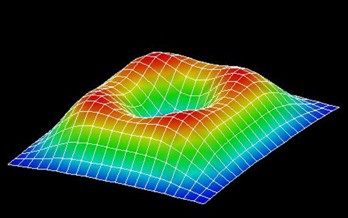
This leads to an additional confinement in addition to the wire potential.
However, for the first and forth eigenstate, the confinement does not play an
important role whereas for the second and third it does. The effect is more
dominant onto the wave functions but not so pronounced onto the values of the
eigenenergies. Now the degeneracy of the 2nd and 3rd
eigenstate is slightly lifted in comparison to the case where no magnetic field
is applied.
 |
 |
|
1st eigenstate: -0.0151 eV |
2nd eigenstate: -0.0375
eV |
 |
 |
|
3rd eigenstate: -0.0378
eV |
4th eigenstate: -0.0602 eV |
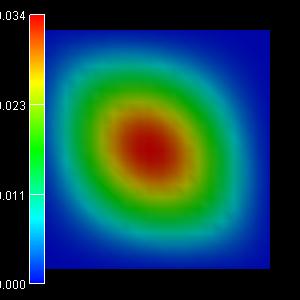
Here, the probabilty density of the second eigenstate is plotted viewed from a
different perspective.
Note: Currently magnetic field only works for option schroedinger-masses-anisotropic =
yes.
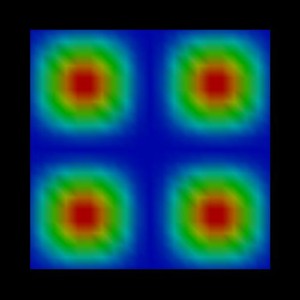
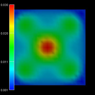
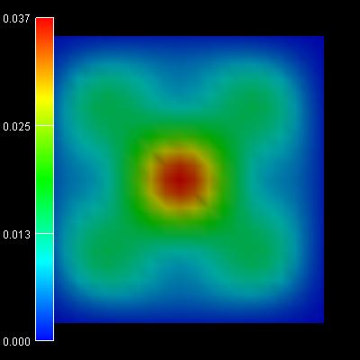
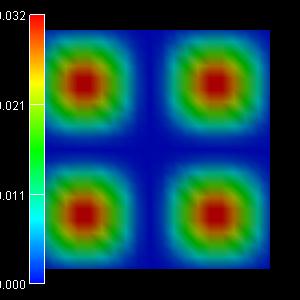
Hole wave functions - 6-band k.p approximation (infinite GaAs barriers)
-> 2Dwire_6x6kp.in
-> 2Dwire_6x6kp_Burt.in
The following figures show the charge densities (Psi²; Psi = hole
wave function) of the four lowest energy confined hole eigenstates in an
infinitely deep 10 nm x 10 nm InAs quantum wire. This time we used 6-band k.p theory to
describe the hole states. Here, the
second and the third eigenstate are no longer degenerate. Only the ground state
looks similar to the single-band effective-mass approximation results.
We used the following Luttinger parameters for InAs:
gamma1 = 20.0, gamma2 = 8.5, gamma3
= 9.2
This corresponds to the Dresselhaus parameters L, M, N:
L = -55, M = -4, N = -55.2
6x6kp-parameters = -55.000d0 -4.000d0
-55.200d0 ! L, M, N [hbar^2/2m](--> divide by hbar^2/2m)
0.39d0
! delta_split-off [eV]
 |
 |
|
1st /2nd eigenstate:
-0.0342 eV |
3rd/4th eigenstate:
-0.0367 eV |
 |
 |
|
5th/6th eigenstate:
-0.0557 eV |
7th/8th eigenstate:
-0.0581 eV |
The energies are contained in this file:
ev_hl_6x6kp_qc001_num_kpar001_2D.dat
num_ev: eigenvalue[eV]: cb:
hh: lh:
s/o:
1 -0.34226968E-01
0.000E+00 0.894E-01 0.905E+00 0.519E-02
2
-0.34226968E-01 0.000E+00 0.894E-01 0.905E+00 0.519E-02
3 -0.36675499E-01
0.000E+00 0.285E+00 0.710E+00 0.528E-02
4
-0.36675499E-01 0.000E+00 0.285E+00 0.710E+00 0.528E-02
5 -0.55698284E-01
0.000E+00 0.263E+00 0.718E+00 0.192E-01
6
-0.55698284E-01 0.000E+00 0.263E+00 0.718E+00 0.192E-01
7 -0.58120024E-01
0.000E+00 0.384E+00 0.604E+00 0.113E-01
8
-0.58120024E-01 0.000E+00 0.384E+00 0.604E+00 0.113E-01
We used:
schroedinger-kp-ev-solv =
ARPACK
!
schroedinger-kp-discretization = box-integration
!
kp-vv-term-symmetrization =
yes
! 'yes' (= incorrect physics), 'no'
(= correct physics)
Comment: schroedinger-kp-ev-solv = chearn
leads to very similar (almost identical) results for 6-band k.p
for both options of kp-vv-term-symmetrization =
yes/no.
However, using instead Burt's non-symmetrized discretization
kp-vv-term-symmetrization =
no
! 'yes', 'no'
 |
 |
|
1st /2nd eigenstate:
-0.0383 eV |
3rd/4th eigenstate:
-0.0419 eV |
 |
 |
|
5th/6th eigenstate:
-0.0679 eV |
7th/8th eigenstate:
-0.0768 eV |
num_ev: eigenvalue[eV]: cb:
hh: lh:
s/o:
1 -0.38319736E-01
0.000E+00 0.531E-01 0.941E+00 0.606E-02
2
-0.38319736E-01 0.000E+00 0.531E-01 0.941E+00 0.606E-02
3 -0.41904230E-01
0.000E+00 0.265E+00 0.735E+00 0.860E-03
4
-0.41904230E-01 0.000E+00 0.265E+00 0.735E+00 0.860E-03
5 -0.67878674E-01
0.000E+00 0.414E+00 0.584E+00 0.180E-02
6
-0.67878675E-01 0.000E+00 0.414E+00 0.584E+00 0.180E-02
7 -0.76825362E-01
0.000E+00 0.111E+00 0.874E+00 0.145E-01
8
-0.76825362E-01 0.000E+00 0.111E+00 0.874E+00 0.145E-01
The following is obsolete because the feature
valence-band-masses-from-kp does not really make much sense.
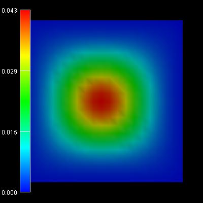
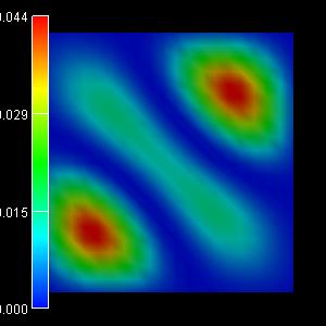
Hole wave functions - Single-band effective-mass approximation (infinite GaAs
barriers)
-> 2Dwire_vbmassesfrom6x6kp.in
Here we use a single-band effective-mass approximation but we use an
effective-mass tensor that is obtained from the Luttinger parameters.
valence-band-masses-from-kp =
yes ! 'yes', 'no'
 schroedinger-masses-anisotropic =
yes ! 'yes', 'no',
'box'
We used the following Luttinger parameters for InAs:
gamma1 = 20.0, gamma2 = 8.5, gamma3
= 9.2
This corresponds to the Dresselhaus parameters L, M, N:
L = -55, M = -4, N = -55.2
 6x6kp-parameters = -55.000d0 -4.000d0
-55.200d0 ! L, M, N [hbar^2/2m](--> divide by hbar^2/2m)


 0.39d0
! delta_split-off [eV]
This leads to the following effective-mass tensor components for the heavy
hole:
mxx = 0.333
myy = 0.333
mzz = 0.333
mxy = -0.943
mxz = -0.943
myz = -0.943
The following figures show the charge densities (Psi²; Psi = hole
wave function) of the five lowest energy confined hole eigenstates in an
infinitely deep 10 nm x 10 nm InAs quantum wire. The degeneracy of the
second and the third eigenstate is now lifted.
 |
 |
|
|
1st eigenstate: -0.0182 eV
(-0.0182) |
2nd eigenstate: -0.0407 eV
(-0.0406) |
|
 |
 |
 |
|
3rd eigenstate: -0.0500 eV
(-0.0500) |
4th eigenstate: -0.0665 eV
(-0.0662) |
5th eigenstate: -0.0896 eV
(-0.0895) |
In the brackets, the eigenvalues for schroedinger-masses-anisotropic =
box are given.
-> 2Dwire_vbmassesfrom6x6kp_iso.in
If we had chosen
 schroedinger-masses-anisotropic = no  !
'yes', 'no', 'box'
then the off-diagonal elements of the effective-mass tensor are not taken
into account.
mxy = -0.943 := 0 <- assumed to be zero!!!
mxz = -0.943 := 0 <- assumed to be zero!!!
myz = -0.943 := 0 <- assumed to be zero!!!
Due to the symmetry of the quantum wire and the effective mass tensor,
the second and the third eigenstate are degenerate.
The relevant wave functions in this case are:
 |
 |
|
1st eigenstate: -0.0186 eV |
2nd eigenstate: -0.0463 eV |
 |
 |
|
3rd eigenstate: -0.0463 eV |
4th eigenstate: -0.0741 eV |
|