www.nextnano.com/documentation/nextnanoplus_tutorials/
nextnano3 - Tutorial
next generation 3D nano device simulator
1D Tutorial
Exciton energy in quantum wells
Author:
Stefan Birner
-> 1DExcitonCdTe_QW.in - CdTe quantum
well with infinite barriers
Exciton energy in quantum wells
This tutorial aims to reproduce the figures 6.4 (p. 196) and 6.5 (p. 197) of
Paul Harrison's
excellent book "Quantum
Wells, Wires and Dots" (Section 6.5 "The two-dimensional and
three-dimensional limits"), thus the following description is based on the
explanations made therein.
We are grateful that the book comes along with a CD so that we were able to
look up the relevant material parameters and to check the results for
consistency.
- In order to correlate the calculated optical transition energies of a 1D
quantum well to experimental data, one has to include the exciton
(electron-hole pair) corrections. In this tutorial we study the exciton
correction of the electron ground state to the heavy hole ground state (e1 -
hh1).
- Bulk
The 3D bulk exciton binding energy can be calculated analytically
Eex,b
= - µ e4 / ( 32 pi² hbar² er² e0²)
= - µ / (m0 er²) x 13.61 eV
where µ is the reduced mass of the electron-hole pair: 1/µ = 1/me +
1/mh
GaAs: 1/µ = 1 / 0.067 + 1 / 0.5 ==> µ = 0.0591
CdTe: 1/µ = 1 / 0.096 + 1 / 0.6 ==> µ = 0.0828
hbar is Planck's constant
divided by 2pi
e is the electron charge
er is the dielectric constant
(GaAs: 12.93, CdTe: 10.6)
e0
is the vacuum permittivity
m0 is the rest mass of the
electron and
13.61 eV is the Rydberg energy.
In GaAs, the 3D bulk exciton binding energy is equal to
-4.8
meV with a Bohr radius of lambda = 11.6 nm.
In CdTe it is equal to -10.0 meV with a Bohr radius of 6.8
nm.
Thus the energy of the exciton, i.e. band gap transition, reads
GaAs: Eex = Egap + Eex,b = 1.519 eV - 0.005 eV
= 1.514 eV.
CdTe: Eex = Egap + Eex,b =
1.606 eV - 0.010 eV
= 1.596 eV.
More details on bulk excitons can be found in Section 6.1 "Excitons in
bulk" (p. 181) of
Paul Harrison's
book "Quantum
Wells, Wires and Dots".
- Quantum well (type-I)
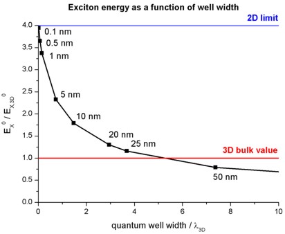
A 1D quantum well for a type I structure has two exciton limits for the ground
state transition (e1-hh1):
- infinitely thin quantum well (2D limit): Eex,qw = 4Eex
lambdaex,qw = lambdaex / 2
- infinitely thick quantum well (3D bulk exciton limit): Eex,qw = Eex
lambdaex,qw = lambdaex
Between these limits, the exciton correction which depends on the well
width has to be calculated numerically, not only for the ground state but also
for excited states (e.g. e2 - hh2, e1 - lh1).
- CdTe quantum well with infinite barriers
In this tutorial we study the exciton binding energy of CdTe quantum wells (with infinite barriers)
as a function of well width.
The material parameters used are the following:
 !-----------------------------------------------------------!

 ! Here we are overwriting the database entries for CdTe.
  !

 !-----------------------------------------------------------!

 $binary-zb-default
  !

  binary-type
  = CdTe-zb-default
  !

  apply-to-material-numbers   = 2
  !

  conduction-band-masses      =
  0.096    0.096    0.096
  ! Gamma      [m0]


  ...


  valence-band-masses         =
  0.6      0.6      0.6
  ! heavy hole [m0]


  ...

  static-dielectric-constants = 10.6
  10.6     10.6       !
We chose infinite barriers, in order to be able to compare the nextnano
calculations with standard textbook results, originally published by G.
Bastard et al. (Phys. Rev. B 26 (4), 1974 (1982)), namely the exciton
binding energy of a type-I quantum well (in units of the 3D bulk exciton
energy Eex, also called effective Rydberg energy) as a
function of well width (in units of the 3D bulk exciton Bohr radius lambdaex).
- Template
The following screenshot shows how to use the Template feature of nextnanomat
in order to calculate the exciton binding energy as a function of the
quantum well width.
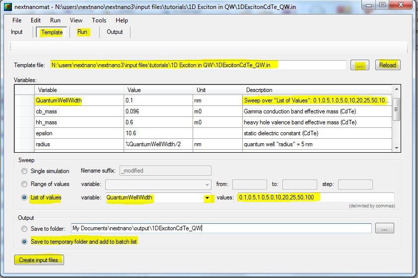
- Open template input file (...).
- Select "List of values", select variable "QuantumWellWidth". The
corresponding list of values are loaded from the template input file.
- Click on "Create input files" to create an input file for each quantum
well width.
- Switch to "Run" and the jobs are executed.
Results
- The following figure shows the exciton binding energy in an infinitely deep
quantum well as a function of well width.
Both quantities are given in terms of the effective Rydberg energy and the
Bohr radius for a 3D exciton in the same material.
Our numerical approach is the following:
The exciton binding energy is minimized with respect to the variational
parameter lambda.
We use a separable wave function:
psi (r) = SQRT(2/pi) 1/lambda exp (- r / lambda)
see e.g. S.L. Chuang, "Physics of Optoelectronic Devices", Wiley, p. 562,
Eq. (13.4.27), Section 13.4.3 "Variational Method for Exciton Problem" or G.
Bastard et al., PRB 26, 1974 (1982)
Thus the 3D limit is not reproduced correctly in our approach (not shown in
the figure).
To obtain the 3D limit, a nonseparable wave function has to be used:
psi (r,ze,zh)
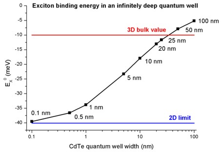
- The following figure shows the exciton binding energy in an infinitely
deep CdTe quantum well as a function of well width.
The nextnano³ results are in nice agreement with the Fig. 6.4 of Paul
Harrison's book although we use a simpler trial wave function with only one
variational parameter.
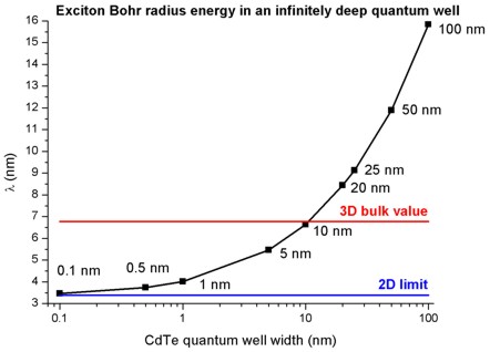
- The following figure shows the exciton Bohr radius lambda in an infinitely
deep CdTe quantum well as a function of well width.
The nextnano³ results for well widths smaller than 10 nm are in nice
agreement with Fig. 6.5 of Paul Harrison's book.
The discrepancy arises because he uses a different trial wave functions (i.e. a
superior approach) with a second variational parameter in addition to lambda.
The 3D bulk value of lambda in CdTe reads: lambdaex = 6.8 nm.
- In order to calculate the exciton correction, the
following
flags have to be used:
 $numeric-control

    simulation-dimension          =
  1
  calculate-exciton
  = yes   !
to switch on exciton
correction
  exciton-electron-state-number =
  1
  !
  exciton-hole-state-number     =
  1     !
- The output of the exciton binding energies can be found in this file:
Schroedinger_1band/exciton_energy1D.dat
The output for the 5 nm CdTe QW looks like this:
 Exciton correction for 1D quantum wells (type-I structures)

 ===========================================================

 static dielectric constant     =
	10.6000000000 []

 effective mass electron        =
	0.0960000000 [m0]

 effective mass hole
	=   0.6000000000 [m0]

 reduced mass
	=   0.0827586207 [m0]

 Bulk Bohr radius of 3D exciton =   6.7778780735
	[nm]

 Bulk 3D exciton energy         =
	-10.0212560410 [meV]


 lambda [nm]        exciton energy
	[meV]   exciton energy [Rydberg]

 0.338893904E+001   -0.158496790E+002
	0.158160603E+001

 ...

 0.421888329E+001   -0.215591082E+002
	0.215133793E+001

 ...

 0.553296169E+001   -0.232757580E+002
	0.232263879E+001

 -----------------------------------------------------------------

 -----------------------------------------------------------------

 Calculated lambda and exciton energy:

 0.546379967E+001   -0.232817837E+002
	0.232324009E+001

 -----------------------------------------------------------------
-23.28 meV for the exciton
binding energy.
"lamba" is the variational parameter which is equivalent to the exciton Bohr
radius in units of [nm].