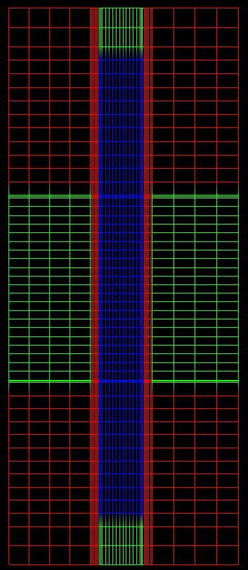
Grid specification
Grid lines (nodes) between explicitly defined grid lines
x-nodes = int1 int2 ...
y-nodes = int1 int2 ...
z-nodes = int1 int2 ...
Grid factors (inhomogeneous grid)
x-grid-factors = double1 double2 ...
y-grid-factors = double1 double2 ...
z-grid-factors = double1 double2 ...
The nodes specified above are distributed according to a geometric series
between the explicitly defined grid lines. The spacing between successive
additional grid lines increases (factor > 1.0) or decreases
(factor <1.0) in the corresponding coordinate axis direction.
(Comment: The term "inhomogeneous" refers to grid lines (=nodes)
between two adjacent grid lines (=x/y/z-grid-lines). However, the
total grid of the whole device is likely to be inhomogeneous in general even if
the grid factor is always 1.0d0.)
Grid type
grid-type = 1 1 1 for xyz-grid
          =
  1 0 1
for xz-grid
            =
  1 1 0
= ...
            =
  1 0 0
The grid type selects by an integer array the coordinate axes relevant for
the present simulation.
This specifier contains redundant information, i.e. the same information as
$simulation-dimension, orientation = ...
which
is now used.
However, the specifier grid-type
must be still there although the values specified here can be arbitrary.
(CHECK: Why?)
force-grid-lines-at-simulation-boundaries = yes ! yes)
= no !
Forces grid lines to exist at minimum and maximum x, y and z coordinates
as specified in $domain-coordinates.
force-grid-lines-at-region-boundaries     =
yes ! (default:
yes)
= no !
Forces grid lines to exist at region boundary coordinates as specified in
$regions.
Grid lines
x-grid-lines = double1  double2  double3 ...
! [nm]
y-grid-lines = double1  double2  double3 ...
! [nm]
z-grid-lines = double1  double2  double3
... ! [nm]
Explicit specification of grid lines for the coordinate directions of the
simulation domain. For each coordinate specified under keyword
$regions there must exist a grid line. In
addition to these, one is allowed to specify extra grid lines. At material
boundaries there must be a grid line (or a grid line determined by an
appropriate number of nodes specified in the following).
Grid lines (nodes) between explicitly defined grid lines
x-nodes = int1 int2 ...
y-nodes = int1 int2 ...
z-nodes = int1 int2 ...
Between each grid line there are a certain number of nodes. One node is a
kind of grid line.
(The final grid which is called physical grid, consisting of grid lines and
nodes is being transformed to the material grid (volume grid). A material grid
point is placed exactly in between two physical grid points. The physical grid is
being discretized to solve for
instance the Poisson equation.
More
information on grids ...)
Subregions, specified by grid lines above,
must be on a grid line of the final grid.
Add int1, int2, ... grid lines between two explicitly specified grid lines
above. Between any explicitly defined pair of gridlines, the number of
additional nodes must be specified, even if zero grid lines (nodes) have to be
added.
All our equations are numerically solved on a discrete grid,
i.e. for each node (i.e. grid-lines and nodes) a value
for the electrostatic potential and the wave function amplitudes is calculated.
(Even in nature the crystal is not a continuum but is made from discrete
atoms.
For a distance of 1 nm, 7 nodes correspond to a grid spacing of 0.142 nm which
is also the distance of two neighboring atoms in graphene.
The nearest neighbor distance in diamond is 0.154 nm.
The nearest neighbor distance in silicon is 0.235 nm.
The lattice constant in silicon is 0.532 nm.)
In each direction at least three grid points have to be defined,
e.g. one grid line (x-grid-lines) +
one node (x-nodes) + one
grid-line (x-grid-lines) = 3 grid points.
Grid factors (inhomogeneous grid)
x-grid-factors = double1 double2 ...
y-grid-factors = double1 double2 ...
z-grid-factors = double1 double2 ...
Grid coarsening factors in subregions. The grid factor is the exponent of a
geometric series.
The nodes specified above are distributed according to a geometric series
between the explicitly defined grid lines.
The spacing between successive
additional grid lines increases (factor > 1.0) or decreases
(factor <1.0) in the corresponding coordinate axis direction.
A geometric factor of 1.0 is the equivalent of equal spacing.
(Comment: The term "inhomogeneous" refers to grid lines (=nodes)
between two adjacent grid lines (=x/y/z-grid-lines). However, the
total grid of the whole device is likely to be inhomogeneous in general even if
the grid factor is always 1.0.)
In a geometrically spaced region, the distance between two consecutive nodes changes by the grid factor (rate of change or common ratio).
For instance, with a geometric factor of 2.0, the largest division is twice the length of the previous division,
which is twice the length of the division before that, ...
Example:
  x-grid-lines   = -32.0
0.0   32.0  ! [nm]

  x-nodes        =
31    31

  x-grid-factors =      0.5
2.0
The grid lines will be positioned at
  -32.0  -16.0  -8.0  -4.0  -2.0  -1.0
-0.5  -0.25  -0.125  -0.0625  ...  0.0  ...
4.0  8.0  16.0  32.0
So the common ratio is 0.5 and
2.0, i.e. the values are half the
value of the previous one (from -32.0 to 0.0 and
twice the value of the previous one (from 0.0 to 32.0).
0.5 and
2.0 are usually too "large". It is best to
use values such as 0.95 or
1.05 that are closer to an equally spaced
grid (1.0).
!-------------------------------------------------------------

   ! Define the distance between the two neighboring grid lines.

   !-------------------------------------------------------------

   distance         = coordinate_max - coordinate_min

   coordinate_delta = distance * (gridfactor - 1.0) / (gridfactor**(nodes+1) - 1.0)


  DO k=1,nodes

   coordinate       = coordinate_min + coordinate_delta * (gridfactor**k - 1.0) / (gridfactor - 1.0)

  END DO